Principal Component Analysis

PCA is a data transformation technique.

Given an n-dimensional set of data points, it finds an n-dimensional orthonormal basis aligned with the directions along which the data varies the most.

Besides computing the n basis axes, PCA also computes n values which tell how much of the total variance in the dataset is captured by each axis.

Example 2D dataset

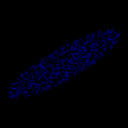
To illustrate this post we will be using a 2D dataset made of 1024 points uniformly distributed in the shape of an ellipse of radii \(a=1\) and \(b=.25\). The ellipse is centered at \((.5,.5)\) and tilted by \(\frac{\pi}{6}\) radians.

Simple Linear Regression

First, let’s detour a little to talk about Simple Linear Regression, which is a basic method one can use to approximate a set of 2D data points with a best fitting line.

It is common practice to define the best fitting line using ordinary least squares. i.e., the line that minimizes the sum of vertical distances between itself and the points in the dataset.

I hope that the below video depicts this idea clearly:

The vertical distances (also called residuals) are in yellow. As the best fitting line candidate (in white) rotates the plot at the bottom represents the OLS sum. It can be seen that the sum goes to infinity when the line is vertical, but reaches a minimum when the line is as tilted as the dataset.

In our dataset these calculate to \(\widehat\alpha=.238\ldots\) and \(\widehat\beta=.523\ldots\) which we can plug in the line equation:

\(.523\ldots=\widehat\beta\simeq tan(\frac{\pi}{6})=.577\ldots\) which means that the slope of the best fitting line is about \(\frac{\pi}{6}\) radians, like our dataset. All good.

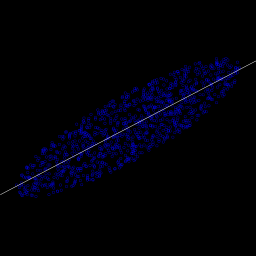
The point of this detour is to introduce SLR as a basic intuitive method to capture some meaningful feature of an arbitrary dataset using a much simpler instrument such as a line.

Principal Component Analysis

PCA can be seen as a generalization of the above. Instead of minimizing the vertical distances to a candidate line, it minimizes the perpendicular ones, and instead of stopping at a single line it produces a whole orthonormal basis.

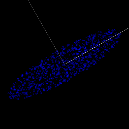
The algorithm itself is short: center the dataset by subtracting its mean, build the covariance matrix of the centered data, and eigen-decompose it. The resulting eigenvectors are the principal axes, and each eigenvalue is the variance captured by its axis. Sorting the eigenvalues in decreasing order sorts the axes from most to least informative.

Practical uses of PCA

Most of the time, PCA is used as a preceding step to data reduction. Since PCA provides a set of axes where the dataset projections are sorted in decreasing order of variance, you can say that the amount of information provided by each new axes is less and less.

Actually, you may drop some of the trailing axes and obtain a dimensionally-reduced (and hence more tractable) version of your dataset that roughly captures the same amount of information as the original dataset.

Data visualization

A classic use is to drop all dimensions but the first two or three in order to plot the dataset in 2D or 3D. With a little luck, a heavy multi-dimensional dataset will exhibit some sort of obvious clustering you can make sense of when drawn on screen.

Machine Learning

For ML, clustering, … it makes sense to run PCA on your data first. Then drop as many trailing principal components while still preserving the maximum amount of information (e.g. setting a cutoff at 99%). And from that moment on, work with the dimensionally-reduced dataset.

Physics

There is a beautiful relationship between the PCA of a set of points (interpreted as masses) and the tensor of inertia of said masses.

The principal axes that PCA finds for a set of points interpreted as masses are precisely the principal axes of inertia of that body. This has a neat practical consequence: when a body spins about one of its principal axes, its angular momentum and its angular velocity are parallel, which is exactly the condition for it to rotate without wobbling.

PCA implemented in Eigen

This is the implementation of PCA I am using in my code since I decided to replace some legacy implementations of numerical algorithms by Eigen.

Eigen::MatrixXd M;

M_to_E( m_M, __out__ M );  // Initialize M with the dataset.

const Eigen::VectorXd mean = M.colwise().mean();

M.rowwise() -= mean.transpose();

const Eigen::MatrixXd cov  = ( ( M.transpose() * M ) / ( M.rows() - 1 ) );

const Eigen::SelfAdjointEigenSolver< Eigen::MatrixXd > solver( cov );

if ( solver.info() == Eigen::Success )
{
  E_to_M( solver.eigenvalues (), __out__ m_E );  // Collect the solver's result.
  E_to_M( solver.eigenvectors(), __out__ m_V );	 //
}

YouTube videos

PCA is very well documented on the Internet:

• A great video by Computerphile on PCA.