Spherical Harmonics

Note: This post was written nearly 2 years ago and never published. I’m posting it now as-is, with some sections incomplete but the core content intact.

This post is a quick crash course on what Spherical Harmonics are and how they can be used to efficiently encode and decode incoming radiance (i.e., a spherical view of the scene) at a point.

Motivation

Radiance and irradiance

In the context of rendering:

Radiance (\(L\)) is the amount of light that flows through or is emitted from a point in space in a particular direction.

Irradiance (\(E\)) is the total amount of light energy incident upon a surface at a specific point.

Where:

• \(E\) is the irradiance at a point on the surface.
• \(L(\mathbf{\omega})\) is the radiance arriving from direction \(\mathbf{\omega}\).
• \(\theta\) is the angle between the surface normal and the direction \(\mathbf{\omega}\).
• \(d\mathbf{\omega}\) represents the differential solid angle in the hemisphere of incoming light directions.

Light probes

The definition above talks about surfaces (with a normal). That is, radiance arriving at the point from the positive side of the surface. However, in this post we are interested on the radiance arriving at a point from all directions:

Under certain circumstances we may want to precompute-and-store the incoming radiance \(L\) at a point or a collection of points in the scene in order to approximate illumination dynamically in real-time (possibly making use of \(E\) somehow).

\(L\) is a function defined on the sphere, and is called light probe…

\(E\) shows up in the Rendering Equation but again, in this post we’re only interested in an efficient way to precompute-and-store \(L(\mathbf{\omega})\).

In a real scenario, light probes can be placed either manually or automatically and they are meant to suffciently cover the scene. The goal of each individual light probe is to keep track of what illumination looks like in the volumetric neighborhood of the point they are centered at. Typically, nearby light probes are sampled and the samples obtained are interpolated to figure out the illumination arriving at any given 3D point. This can give a decent and fast-to-query approximation to Global Illumination and/or soft shadowing.

The information stored by a light probe can be pictured of as a panoramic view of what the point sees around itself. So typical ways to initialize (or update) a light probe are to literally render/rasterize the scene around (maybe with 6 cubemap-arranged cameras) or ray-tracing the surroundings stochastically.

Whichever the method, the resulting irradiance is a spherical collection of colors-and-their-magnitudes. Or, in better words, a function defined on the sphere which yields a color when evaluated at each unit direction. Which, in more humane terms, is a \(360\deg\) photograph of the scene from the point (a panorama or a cubemap if you prefer).

Those are usually rather heavy, and since scenes typically require (many) thousands of light probes to sufficiently cover their volume, finding a highly efficient and performant (albeit lossless) way to encode such spherical color maps sounds ideal.

It is important to note that such radiances-arriving-at-a-point maps can be very high-frequency as soon as we involve high-intensity point lights (such as the sun) and hard shadows. So in some engines all direct lighting coming from hard lights is calculated dynamically and light probes are used exclusively for indirect illumination and soft shadowing, which is much lower frequency.

So let’s establish the goal of this post as:

Find a highly efficient/performant way to encode (low-frequency) spherical color maps with as little loss as possible.

Cubemaps

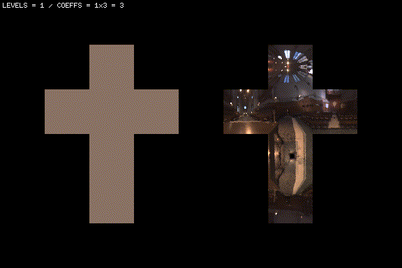
Throughout this post I will display \(L(\mathbf{\omega})\) as cubemaps because cubemap projections exhibit little distortion compared to angular or latitude-longitude maps.

It is important to note that in doing so, the integrals we will be calculating below need to account for distortion in their differential element.

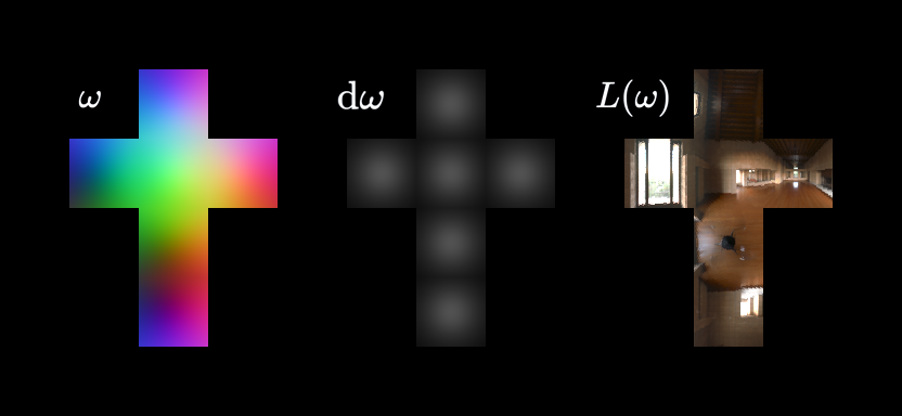
The rgb-coded cubemap represents all the unit directions in a sphere \(\mathbf{\omega}\). The grayscale cubemap represents the differential element conversion between the unit sphere and the unit cubemap \(\mathrm{d}\mathbf{\omega}\). The HDR map unfolded as a cubemap is an example of an incoming radiance map \(L(\mathbf{\omega})\).

Sanity check: The sum of all the grayscale patches must be \(4\pi\) = the surface of the unit sphere.

Spherical Harmonics

SHs have no particular connection with rendering or radiance encoding. They are a generic mathematical contraption with which you can project some input data given in an input realm (usually space) onto another realm (usually frequency-related). This projection process is also reversible, which allows for encoding/decoding.

This is all quite reminiscent of the Fourier Transform & Co..

SH are particularly interesting in the context of Computer Graphics because their domain is the unit sphere, which makes them ideal to encode directional information, such as light probes as described above.

Orthogonality and Key Properties

Spherical Harmonics have several mathematical properties that make them ideal for encoding spherical functions:

Orthogonality: The SH functions are orthogonal over the sphere. This property allows us to decompose any spherical function into independent components without interference between different harmonics.

Completeness: Any square-integrable function on the sphere can be represented as a linear combination of spherical harmonics. For rendering, this means we can approximate any incoming radiance distribution to arbitrary precision by using enough SH coefficients.

Rotation Invariance: The total power in each frequency band (each level \(l\)) is preserved under rotation. This makes SH coefficients stable when objects or light probes are rotated.

Frequency Separation: Lower-order harmonics capture low-frequency (smooth) variations, while higher-order harmonics capture high-frequency (detailed) variations. This natural frequency ordering makes SH perfect for level-of-detail approximations.

From Wikipedia:

“Since the Spherical Harmonics form a complete set of orthogonal functions and thus an orthonormal basis, each function defined on the surface of a sphere can be written as a sum of these spherical harmonics.”

What the SHs look like

Laplace’s Spherical Harmonics are denoted \(Y_l^m(\omega)\) where:

• \(l\) is called the degree or order (ranging from 0 to infinity in theory, but we truncate for practical use).
• \(m\) is called the order within degree (ranging from \(-l\) to \(+l\)).

For a given order \(l\), there are \(2l+1\) different harmonics, each identified by a different value of \(m\). This gives us:

• Level 0 (\(l=0\)): 1 harmonic
• Level 1 (\(l=1\)): 3 harmonics
• Level 2 (\(l=2\)): 5 harmonics
• Level 3 (\(l=3\)): 7 harmonics
• Total for \(L\) levels: \(L^2\) harmonics

The harmonics are essentially different “shapes” or “patterns” on the sphere that form an orthogonal basis. Below is my implementation for the first 4 levels

static constexpr T m_k01 = 0.2820947918;  // sqrt(  1/pi)/2.
static constexpr T m_k02 = 0.4886025119;  // sqrt(  3/pi)/2.
static constexpr T m_k03 = 1.0925484306;  // sqrt( 15/pi)/2.
static constexpr T m_k04 = 0.3153915652;  // sqrt(  5/pi)/4.
static constexpr T m_k05 = 0.5462742153;  // sqrt( 15/pi)/4.
static constexpr T m_k06 = 0.5900435860;  // sqrt( 70/pi)/8.
static constexpr T m_k07 = 2.8906114210;  // sqrt(105/pi)/2.
static constexpr T m_k08 = 0.4570214810;  // sqrt( 42/pi)/8.
static constexpr T m_k09 = 0.3731763300;  // sqrt(  7/pi)/4.
static constexpr T m_k10 = 1.4453057110;  // sqrt(105/pi)/4.

static T Y_0_0( const V3_t&   ) { return    m_k01; }

static T Y_1_0( const V3_t& n ) { return ( -m_k02 * n.y ); }
static T Y_1_1( const V3_t& n ) { return (  m_k02 * n.z ); }
static T Y_1_2( const V3_t& n ) { return ( -m_k02 * n.x ); }

static T Y_2_0( const V3_t& n ) { return (  m_k03 *               n.x * n.y                         ); }
static T Y_2_1( const V3_t& n ) { return ( -m_k03 *               n.y * n.z                         ); }
static T Y_2_2( const V3_t& n ) { return (  m_k04 *       ( ( 3 * n.z * n.z ) -   1               ) ); }
static T Y_2_3( const V3_t& n ) { return ( -m_k03 *               n.x * n.z                         ); }
static T Y_2_4( const V3_t& n ) { return (  m_k05 *       ( (     n.x * n.x ) - ( n.y * n.y     ) ) ); }

static T Y_3_0( const V3_t& n ) { return ( -m_k06 * n.y * ( ( 3 * n.x * n.x ) - ( n.y * n.y     ) ) ); }
static T Y_3_1( const V3_t& n ) { return (  m_k07 * n.z * ( (     n.y * n.x )                     ) ); }
static T Y_3_2( const V3_t& n ) { return ( -m_k08 * n.y * ( ( 5 * n.z * n.z ) - ( 1             ) ) ); }
static T Y_3_3( const V3_t& n ) { return (  m_k09 * n.z * ( ( 5 * n.z * n.z ) - ( 3             ) ) ); }
static T Y_3_4( const V3_t& n ) { return ( -m_k08 * n.x * ( ( 5 * n.z * n.z ) - ( 1             ) ) ); }
static T Y_3_5( const V3_t& n ) { return (  m_k10 * n.z * ( (     n.x * n.x ) - (     n.y * n.y ) ) ); }
static T Y_3_6( const V3_t& n ) { return ( -m_k06 * n.x * ( (     n.x * n.x ) - ( 3 * n.y * n.y ) ) ); }

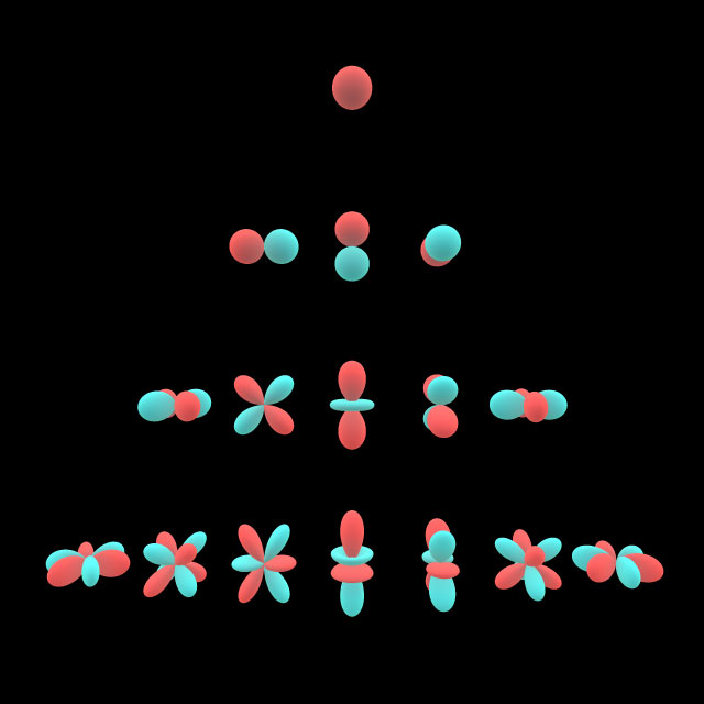
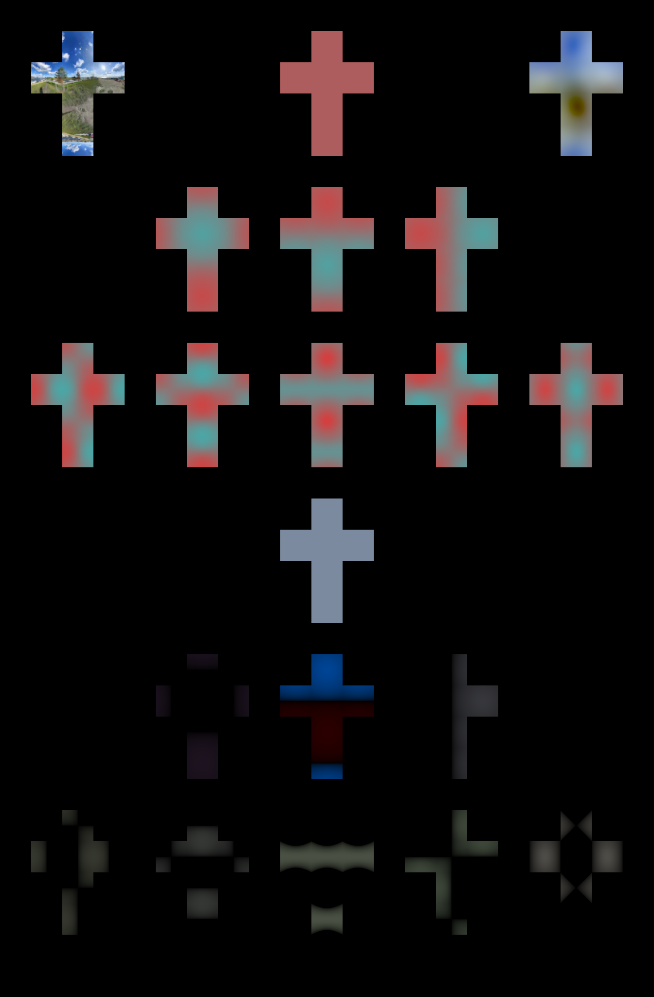
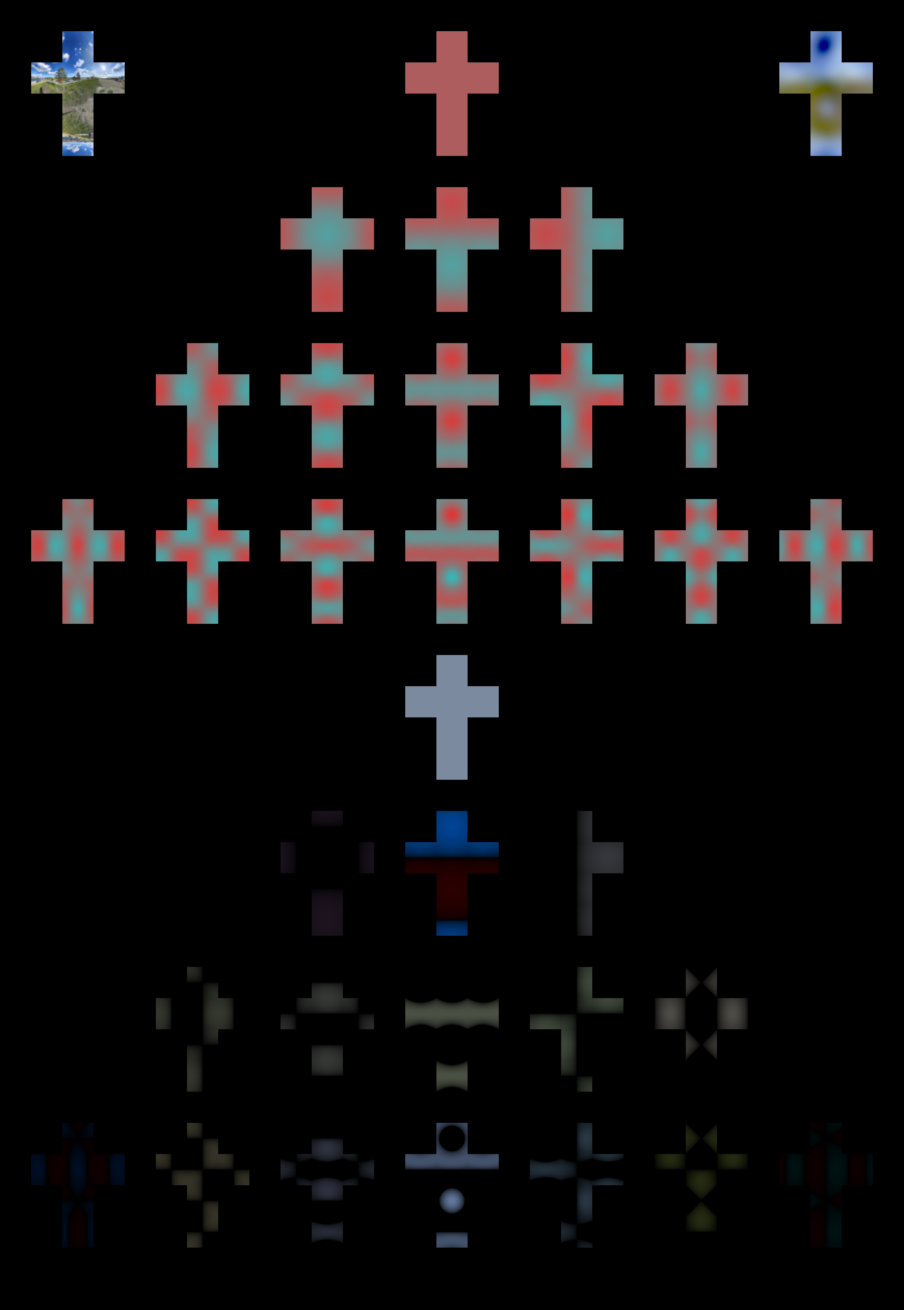
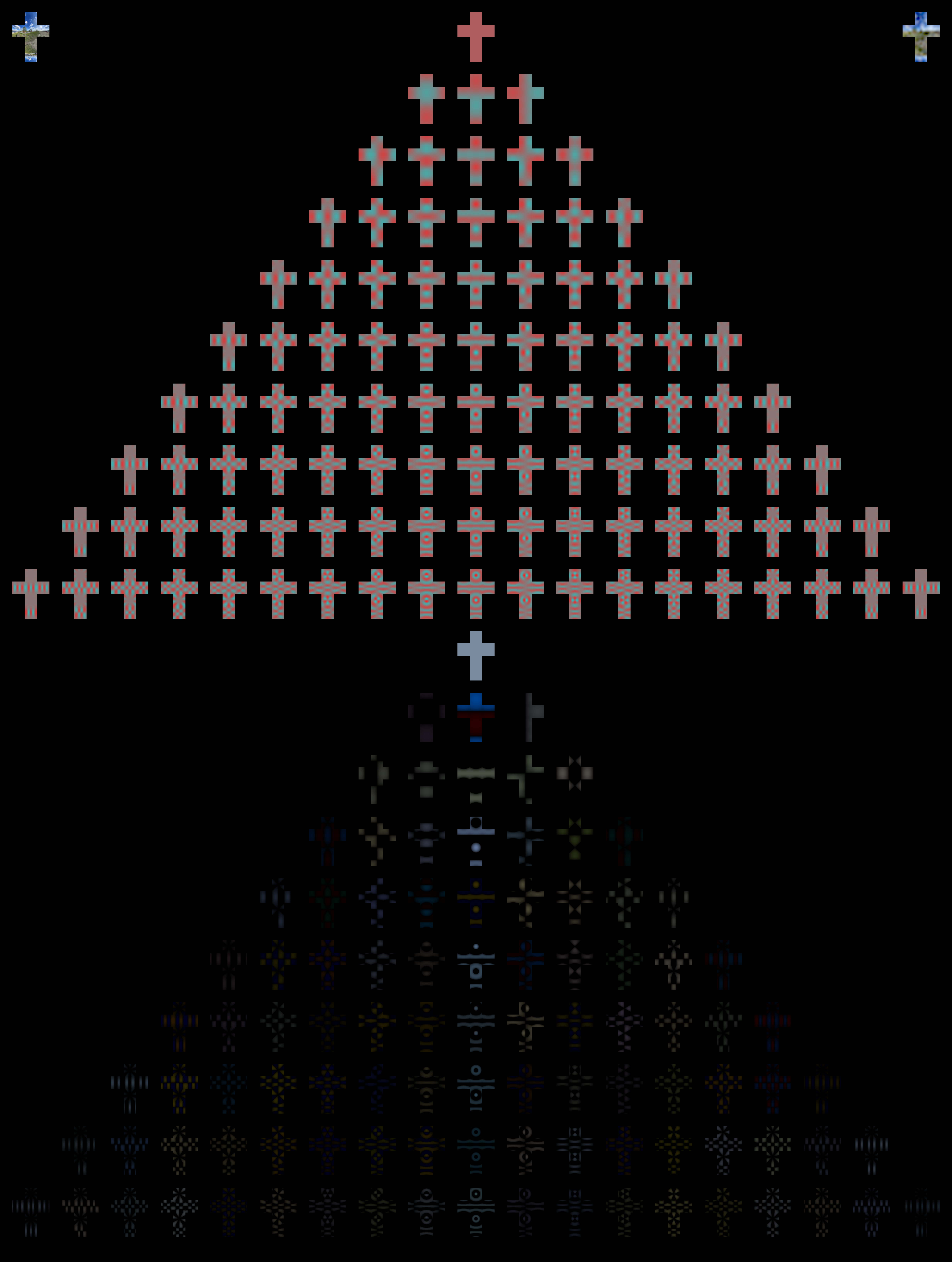
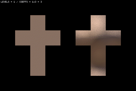
This spherical (i.e., polar in 3D) plot represents the SH basis for the first four levels (L0-L1-L2-L3). The SH magnitude is used for the radius at each spherical coord and the sign is used for the color.

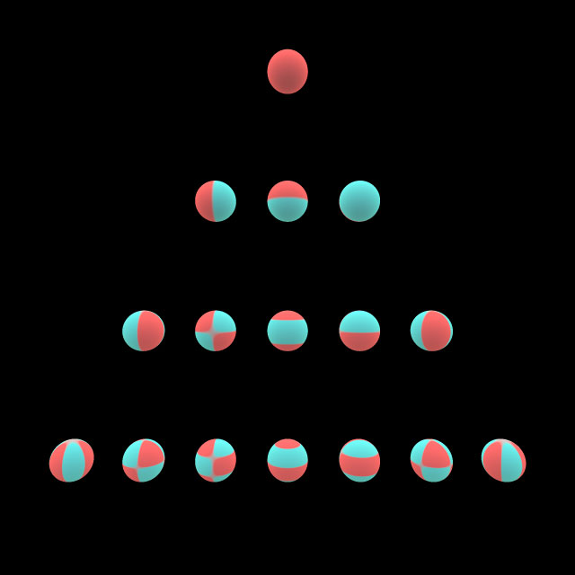
This is the same type of plot, but fixating \(r=1\) and using the magnitude/sign to interpolate between both colors. Note that I have thresholded the magnitude a bit so sign-flip boundaries more sharply distinct.

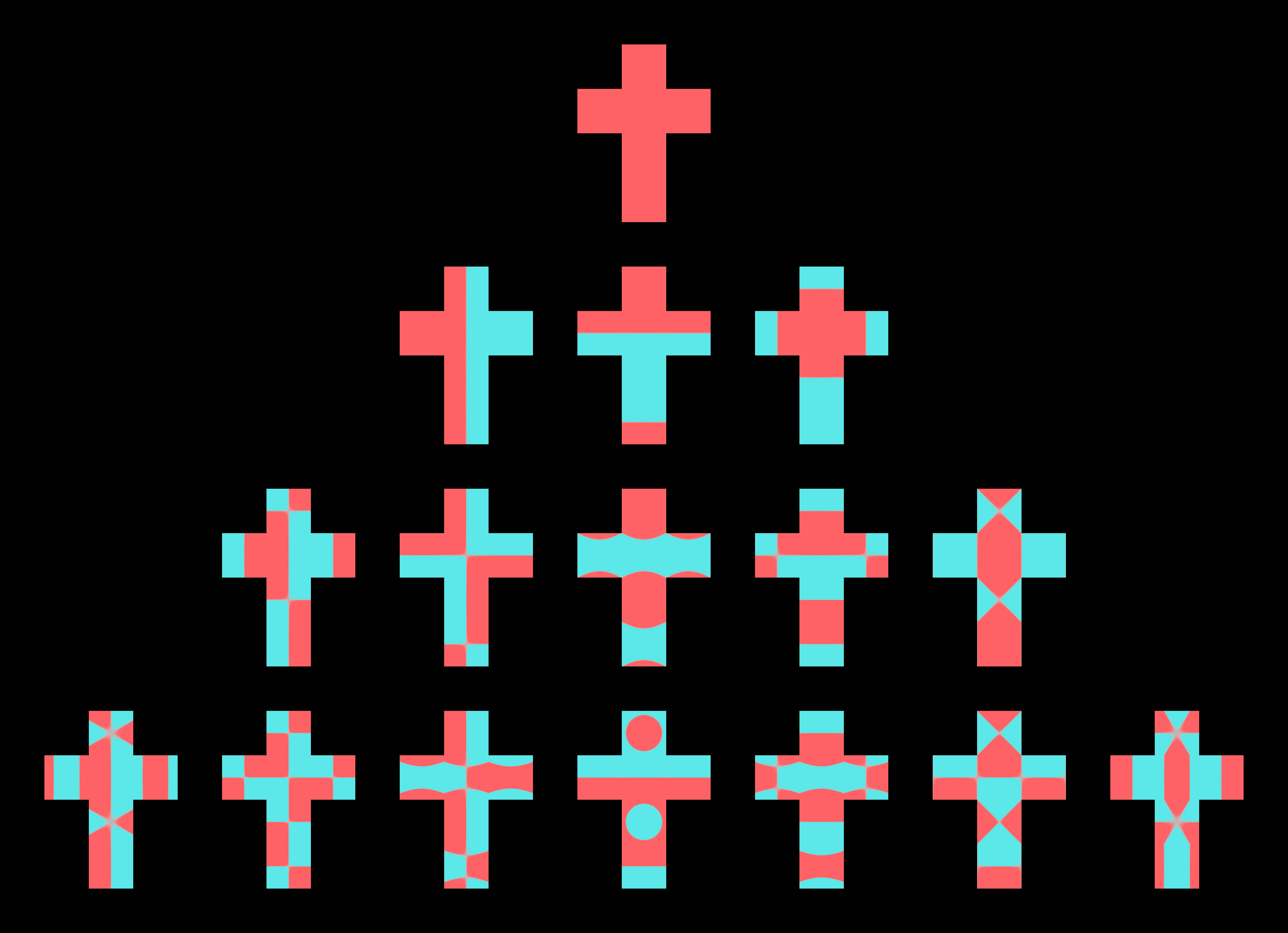
This is again the same plot, but now each unit sphere is unfolded in a cubemap layout. The same color thresholding is used here.

What the SHs will do for us

Recap: The radiance arriving at a point from all directions is a fundamental building block in many real-time GI approximation algorithms. Let’s use the term light probe from now on.

A light probe stores what a point in space sees if it looks around. In other words, a light probe is nothing but a render of the scene with a spherical cam centered at the point.

The radiance arriving at a point from all directions is precisely a (color) function defined on the surface of a sphere centered at the point. Thus, we can encode arriving directional radiance with SHs.

Encoding/Decoding

Let’s define some terminology here:

L: Number of SH levels we will use.

Each level contributes \(L+1+L\) SHs.

So, for example, if we choose \(L=4\), then the total number of SHs involved will be \(N_{SH}=1+3+5+7=16\). It can be easily proven that for any \(L\), the total number of SHs will be \(N_{SH}=L^2\).

Encoding: The process of projecting the input panorama onto each of the \(N_{SH}\) harmonics. This process yields exactly \(N_{SH}\) real coefficients.

Decoding: The process of restoring the input panorama with the linear combination of those \(N_{SH}\) real coefficients each multiplied by its corresponding harmonic.

SH codec: This is the shortname with which we will refer to the process of encoding-and-decoding an input panorama.

Naturally, the higher the number of levels \(L\) the lower the loss of information. But also the number of coefficients (storage and mathematical operations required) will grow quadratically.

For light probes in real-time \(L=3\) or \(L=4\) are usual choices. Radiance arriving at a point is hoefully low-frequency, so few coefficients offer a good compromise between detail preservation and storage size.

It goes without saying, but the SH codec is called once per color component (i.e., \(3\) times per component). This also means that the actual number of real coefficients for a color input panorama is \(3L^2\).

LDR panorama

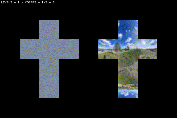
Let’s start with this panorama taken from commons.wikimedia.org. The image is 8-bit, Low-Dynamic-Range, and not particularly high-frequency. i.e., a 360-degree panorama of a pretty exterior.

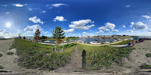
Here’s what happens if we pass it through our SH codec with \(L=3\) (\(9 \times 3=27\) coefficients).

Now with \(L=4\) (\(16 \times 3=48\) coefficients).

And now with \(L=10\) (\(100 \times 3=300\) coefficients).

You can right-click and download (or open in another tab) to view these images at 1:1 scale.

The more the SHs (and coefficients) the more faithful and detailed the reconstruction becomes. While this is obvious, it is important to remark that the SH basis we’re using is “ordered by frequency”, meaning that the first ones encode lower-frequency bands, and adding more and more SHs adds more and more higher-frequency bands. In the continuous case, an infinite number of SHs and coefficients would be required to guarantee an ever lossless restoration. In the discrete case, as with the FT and other transforms, a finite amount of coefficients (proportional to the input data size) will suffice.

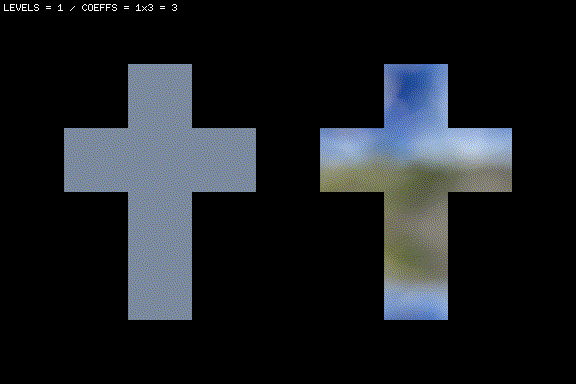
Let’s try with a spherically-blurred version (not a regular image blur):

The most important takeaway here is:

With just a handful of floating-point coefficients we are able to reconstruct a decent low-frequency approximation to an arbitrarily large-resolution panoramic view of a scene. The encoding/decoding process is defined by a very compact and fairly efficient formulation.

Now, how well-behaved an SH codec is? Does it also work well with more complicated data?

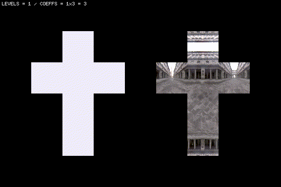
HDR panorama

Since an SH codec transforms data from its natural space domain to the frequency domain, one can reasonably expect that the type of frequencies found in the original data will greatly affect the amount of SH levels (coefficients) necessary to reconstruct data more or less faithfully.

Meaning that data with higher frequencies will be encoded at a greater loss. This sounds intuitive. But there is other less obvious and more harmful implication. As soon as high frequencies appear in the data, artifacts (and not just a loss of detail) will start to appear. Ringing in particular.

This is nothing but a manifestation of the well-known Gibbs phenomenon.

Higher frequencies in an image semantically mean more fine/sharp detail (i.e., more average variation from one pixel to its neighbors). But another factor that amplifies the amount of variation is the dynamic range of the data. Having a high-dynamic range may or may not affect what frequencies are present, but will certainly affect the amplitudes (the magnitude) of the encoded coefficients. Since the harmonics are wave-like, ringing may occur.

The only true solution to this problem would be to keep adding more and more levels/coefficients. But that is obviously not an option. So we may be forced to cheat a little:

• Reduce or clamp the dynamic range (HDR->LDR).
• Blur the input data to shave off the higher frequencies.

Let’s try with another classic HDR panorama. High-frequencies and high-amplitudes together cause a wobbly disaster:

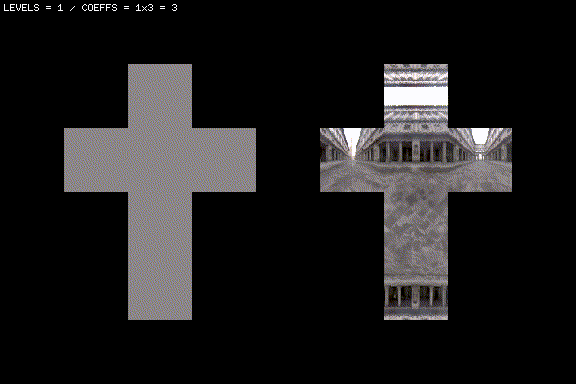
And now let’s try with a spherically-blurred version of the same map. The particular blur I am using here is a cosine-weighted hemispherical blur:

Because type of blur used is cosine-weighted over the hemisphere, this light probe exactly captures the irradiance that a lambertian surface would receive from the scene if illuminated with the unblurred HDR panorama.

And this is precisely what SH encoding/decoding is good for:

Valuable resources

These are “mandatory” resources with great in-depth explanations:

• Stupid Spherical Harmonics Tricks by Peter-Pike Sloan.
• An Efficient Representation for Irradiance Environment Maps by Ramamoorthi and Hanrahan.
• Spherical Harmonic Lighting: The Gritty Details by Robin Green.