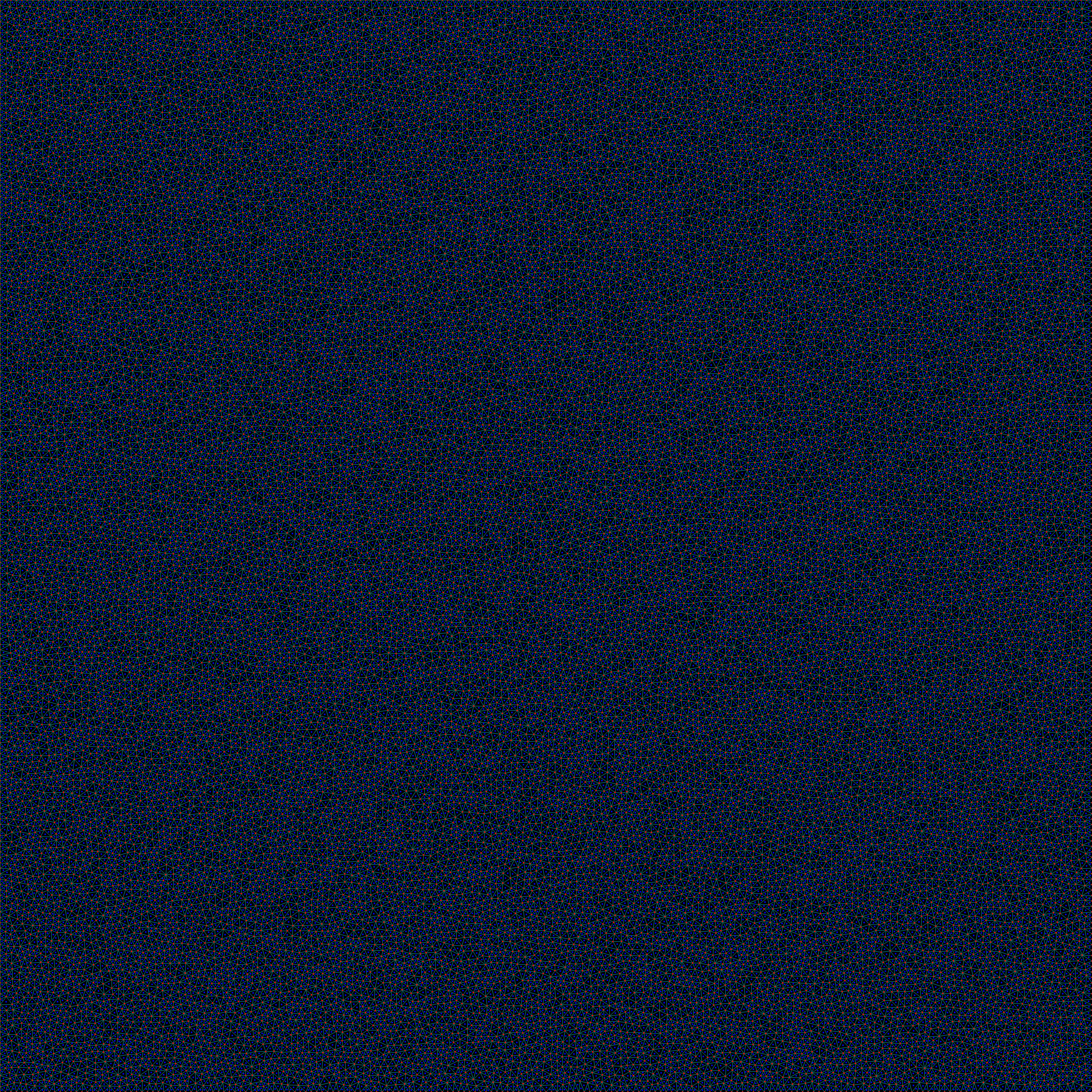
Procedural Island Generation (I)

This post marks the beginning of a series on procedural island generation. I recently fell in love with Amit Patel’s brilliant polygon map generation articles, and this series will be my own exploration and interpretation of those techniques.

This series assumes familiarity with computational geometry and procedural generation concepts such as Delaunay triangulation, Voronoi diagrams, Simplex noise, etc…

To challenge myself (I’m usually a C/C++ person), I decided to implement this in Rust. But I will barely delve into implementation details though. This series will focus on the algorithm itself, with neat (hopefully!) visualizations of the intermediate calculations.

Motivation

The main reason why I am tinkering with terrain generation now is Strike Back, the flight sim I’ve been developing on and off. I will be using this algorithm as a foundation to create battle arenas, and plan to extend it eventually.

Working Domain

Procedural terrain generation offers infinite variety from finite code. But islands make particularly interesting subjects because they’re self-contained worlds with natural boundaries. The polygon-based approach we’ll explore provides a nice balance between organic appearance and computational tractability.

We’ll work in a regular grid within a unit square domain. While regular grids are the classic approach for terrain generation (much simpler implementation, no topological headaches), irregular grids produce far more organic-looking geometry. That’s what we’re after.

Irregular grids have been having a moment lately, BTW. Especially since Townscaper captured everyone’s imagination.

Seed Point Generation

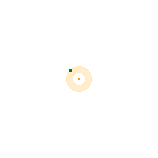
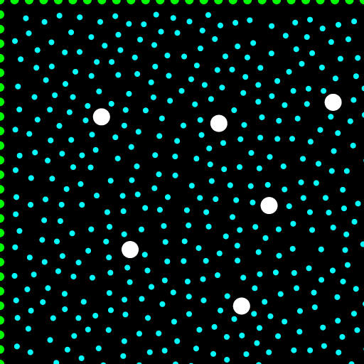
The foundation of an organic-looking terrain mesh is the distribution of its vertices. Random point placement leads to ugly, irregular triangulation. We need something better. Ideally, we need points that are random yet evenly spaced. This is where blue noise comes in.

Blue Noise and Poisson Disk Sampling

Blue noise distributions have a specific property: points maintain a minimum distance from each other whilst filling space uniformly. No clumping, no voids. The spectrum of blue noise is weighted toward higher frequencies, which translates visually to pleasant, nature-resembling distributions.

Bridson’s algorithm for Poisson disk sampling is elegantly simple:

1. Start with a random initial point
2. Generate candidate points in an annulus around existing points
3. Accept candidates that are far enough from all existing points
4. Repeat until no valid candidates remain

The key parameters are:

• \(r\): minimum distance acceptable between points
• \(k\): number of candidates to try before rejection (typically 30)

The algorithm maintains an “active list” of points that might still have valid neighbors. When a point fails to produce valid candidates after \(k\) attempts, it’s removed from the active list.

Spatial indexing is crucial for efficient nearest-neighbor queries in Bridson’s algorithm. A simple grid works well: divide space into cells of size \(r/\sqrt{2}\), ensuring at most one point per cell for \(O(1)\) lookups.

Below is an auxiliary visualization animation I wrote in Python:

Lloyd’s Relaxation

There are different families of algorithms for blue noise generation. Dart-throwing methods, void-and-cluster, Fourier-based methods, relaxation methods, …

While we will stick to Bridson’s algorithm as described above, I am fond of Lloyd’s relaxation (also known as Voronoi iteration). And because we will be working with the Voronoi diagram later I thought it would be worth mentioning.

The process is beautifully simple:

1. Start with any set of random points.
2. Compute the Voronoi diagram for current points
3. Move each point to the centroid of its Voronoi cell
4. Repeat until convergence

This iterative process naturally evolves toward a hexagonal-dominant grid; the most efficient packing in 2D.

Below is another animation I made in Python:

Lloyd’s relaxation is computationally expensive and produces overly regular distributions that can look artificial for terrain. Bridson strikes a better balance: it’s fast and maintains the organic irregularity we want.

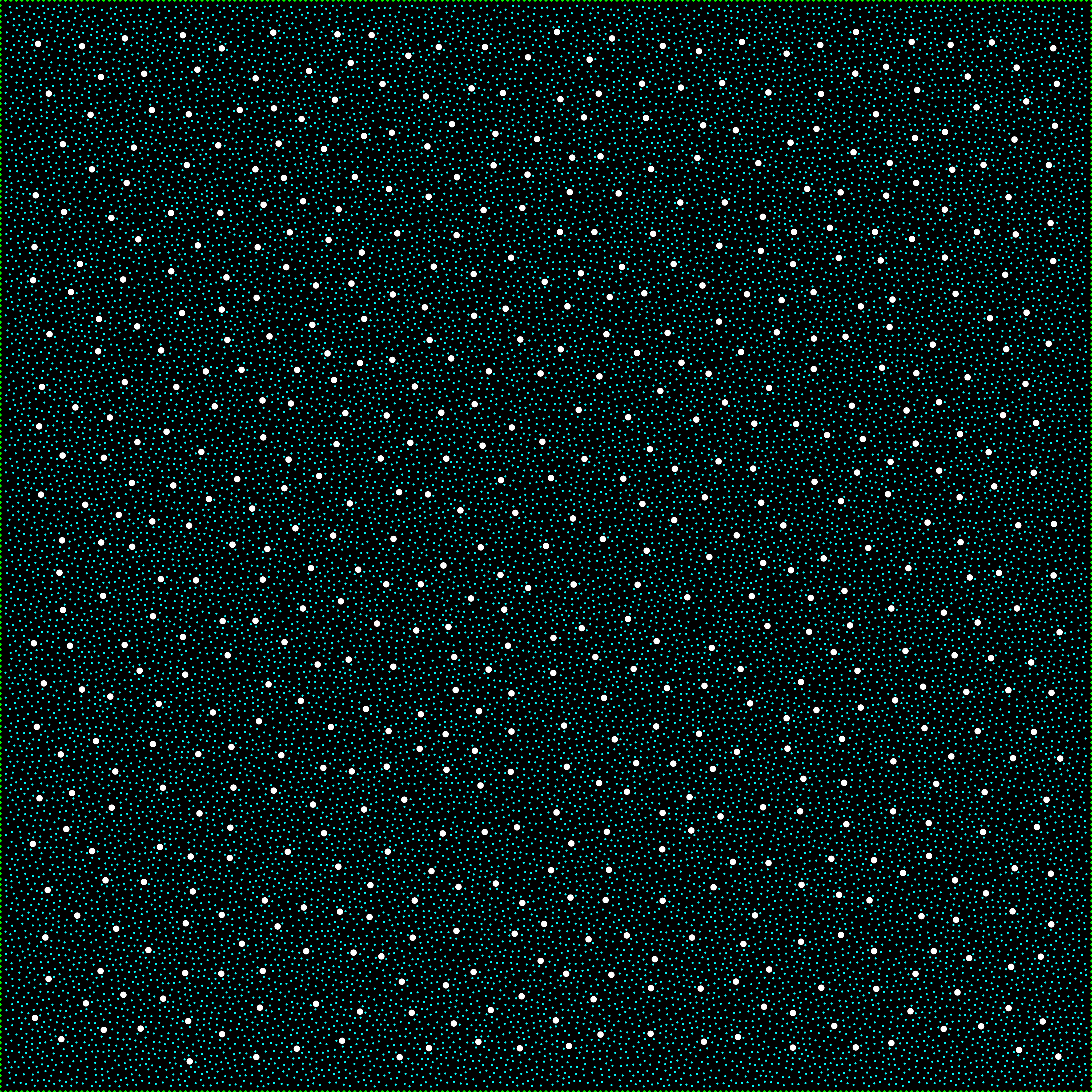
Boundary Treatment

Instead of letting Poisson disk sampling run across the entire domain, I restrict it to a shrunk area, leaving a gap of radius \(r\) around the edges. Then I add two rings of evenly-spaced points: one at the boundary itself (green), and another ring \(r\) units outside the domain (red).

This approach ensures full coverage with well-behaved triangles at the edges for Delaunay triangulation and simplifies handling of unbounded Voronoi regions.

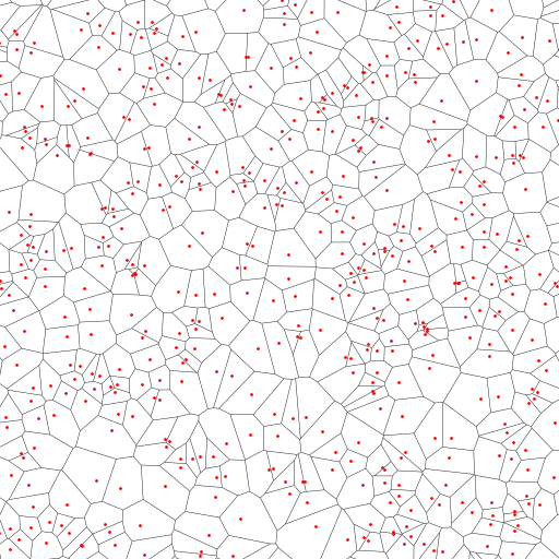
In the animation above, working with a unit square domain and \(r = \frac{1}{200}\), we’d theoretically fit up to \(\left(\frac{1}{r}\right)^2 = 200^2 = 40000\) points in a perfect grid. But Poisson disk sampling produces a looser packing. With the annulus radius range \([r, 2r]\) and rejection sampling, we get ~27000 points in practice, about 68% of the theoretical maximum.

Delaunay Triangulation

With our well-distributed seed points, we need to create a mesh. Delaunay triangulation is the go-to choice for terrain generation because it maximizes the minimum angle of all triangles, avoiding skinny, degenerate triangles that cause numerical and visual issues.

In the visualizations throughout this post, red dots will represent seed points (Delaunay vertices), while blue dots will represent Voronoi vertices (corresponding to Delaunay triangle centers).

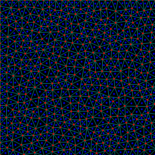
For the implementation, I went with Rust’s delaunator crate. It’s a robust, battle-tested port of the JavaScript library of the same name, implementing a fast sweep-line algorithm that runs in \(O(n \log n)\) time. The cyclic animation is just the same code but decreasing/increasing \(r\) (more/fewer points).

Voronoi Diagram

The Voronoi diagram is the dual of the Delaunay triangulation. Each Delaunay triangle vertex becomes a Voronoi cell, and each Delaunay edge corresponds to a Voronoi edge. For terrain generation, Voronoi cells are a staple: they define convex-shaped regions around each seed point, perfect for assigning terrain properties like elevation, moisture, and biome types.

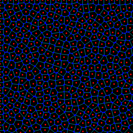
Rather than using an off-the-shelf solution, I built the dual construction using my topology library Topokit, recently ported to Rust. The half-edge (DCEL) data structure I have there makes it trivial to traverse neighbors, and maintain the topological relationships we need for terrain generation. Topokit also handles serialization, relaxation, LOD subdivision, and other features I’ll tap into later.

Circumcenters vs. Centroids

The classical Voronoi diagram uses triangle circumcenters as Voronoi vertices. The circumcenter is equidistant from all three triangle vertices, making it the natural meeting point of three Voronoi cells. However the circumcenter potentially lies outside its triangle if it is obtuse enough. For very flat triangles near boundaries, circumcenters can be far from their triangles, sometimes even outside the domain entirely.

A clever trick I learned from @redblobgames is using triangle centroids instead of circumcenters for Voronoi vertices. This simple change produces smoother, more bubble-like regions with gentler transitions between cells. These softer angles are ideal for terrain generation, and the computation is actually simpler.

Here’s the main takeaway (an animated comparison):

We will go with centroids (instead of circumcenters) all the way through.

Quad Mesh Construction

So we have:

• Red vertices: Original seed points (Delaunay vertices)
• Blue vertices: Voronoi vertices (triangle centers)

Both vertex sets contribute to the final terrain mesh. Throughout this series, we’ll compute attributes like elevation for both red and blue vertices, then triangulate the combined point set to generate the final terrain geometry.

The Red-Blue Pattern

A natural way to combine both the Delaunay and Voronoi meshes is to form quads by each red-blue-red-blue cycle, traversing around shared edges:

1. Start with a Delaunay edge connecting two red vertices
2. This edge is dual to a Voronoi edge connecting two blue vertices
3. The four vertices form a natural quad: red-blue-red-blue

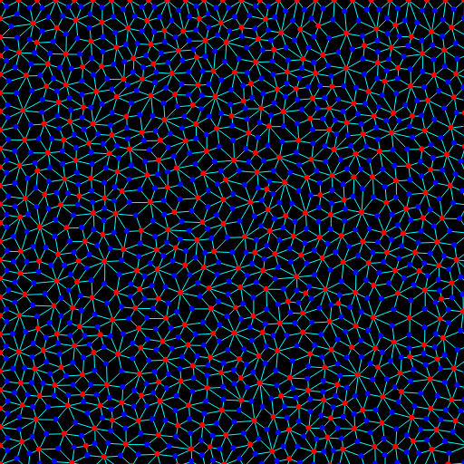
In the resulting quad mesh:

• Red vertices have high valence (many incident edges)
• Blue vertices typically have valence 3 (from triangle origins)
• Edge flow follows a characteristic diamond pattern

Mountain Peak Seed Points

To generate realistic terrain with well-placed mountain peaks, we must flag a special subset of seed points that will become elevation maxima. This two-scale approach ensures mountains maintain natural spacing while aligning perfectly with our existing mesh vertices.

The process leverages a second Bridson’s algorithm run with a much larger radius, typically 4-16 times the original \(r\). This coarse distribution determines where mountain peaks should roughly appear, ensuring they maintain natural spacing across the terrain.

Here’s the algorithm:

1. Build a kD-tree from the fine-grain seed points for efficient nearest-neighbor queries
2. Run Bridson’s algorithm with radius \(R \gg r\) to get coarse peak candidates
3. For each coarse candidate, find its nearest neighbor in the fine distribution
4. Flag these nearest neighbors as mountain peak seeds

Spacial hashing (the kD-tree in my case) is crucial here for performance. With thousands of seed points, nearest-neighbor search would be prohibitively slow otherwise.

This approach has several advantages:

• Natural spacing: Mountains won’t cluster unnaturally or leave large empty regions
• Mesh alignment: Peak points are actual mesh vertices, not interpolated positions
• Controllable density: Adjusting \(R\) directly controls mountain frequency
• Reproducible: Given the same random seed, peak placement is deterministic

These flagged mountain peaks will later serve as local maxima during elevation assignment, with height falloff based on distance. But that’s a topic for Part II.

Above is an animation with varying mountain separation \(R\) over the same set of regular seed points.

Next Steps

This is the distribution (~27000 points) we will be using throughout the rest of the series.

With our mesh structures in place we have the skeletal framework for our island. Part II will dive into elevation assignment using noise functions, creating realistic height maps that produce convincing mountains, valleys, and coastlines.

Resources

• Amit Patel’s Polygon Map Generation - The inspiration for this series
• Bridson’s Original Paper - Fast Poisson disk sampling
• Lloyd’s Algorithm - The mathematical foundation