Procedural Island Generation (IV)

This post is a direct continuation to Part III, where we shaped our terrain with detailed elevation. Now we’ll simulate the complete hydrological cycle: rainfall patterns, river formation, and valley carving through erosion.

Water is the sculptor of landscapes. It carves valleys, deposits sediment, and fundamentally shapes terrain over geological time. While we can’t simulate millions of years of erosion, we can approximate the key processes to create believable drainage patterns.

Hydrological Color Gradients

Before diving into the water simulation, let’s establish the color gradients used to visualize hydrological properties. Each gradient is carefully designed to represent its physical property intuitively:

Key characteristics of each gradient:

• Rainfall uses earth tones transitioning to water colors, matching our intuition about dry vs wet climates
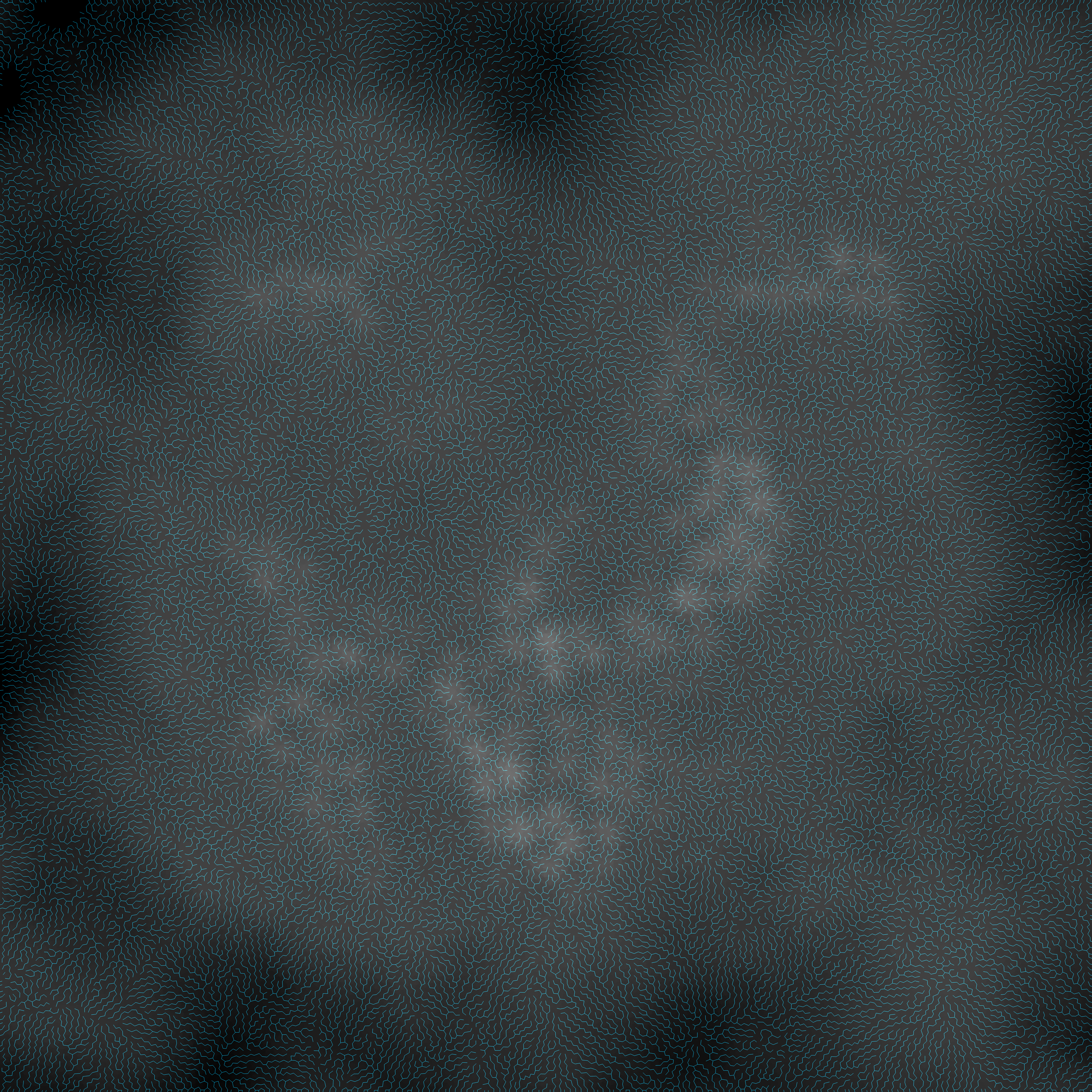
• Humidity employs a temperature-based color scheme, with warm reds for dry air and cool purples for humid conditions
• Moisture features a flat brown segment for arid regions before transitioning through yellow (semi-arid) to green (temperate) to blue (wet)

Slope Assignment

Before water can flow, we need to know which direction is downhill. Our slope assignment seeds a priority queue with ocean triangles (elevation < -0.1) and grows inland. Whenever we pop a triangle, we force every unprocessed neighbour to drain back toward it by storing the twin halfedge as its downslope. The result is a directed acyclic graph that ultimately funnels all triangles to the coast—interior sinks are flattened rather than left as None.

Rainfall Distribution

Rainfall drives the entire water cycle. Rather than uniform precipitation, we want realistic patterns influenced by terrain features. The key insight: mountains capture moisture from prevailing winds.

Orographic Rainfall

When humid air masses encounter mountains, they’re forced upward where cooler temperatures cause condensation. This orographic lift creates heavy rainfall on windward slopes while leaving leeward sides dry—the famous “rain shadow” effect seen in mountain ranges worldwide.

Our implementation simulates this through a wind-ordered traversal of regions:

Wind Ordering

First, we project each region’s position onto the wind direction vector:

πᵢ = pᵢ · w

where w = (cos θ, sin θ) for wind angle θ

Regions are then sorted by their projection value, ensuring upwind regions are processed before downwind ones. This ordering is crucial—it allows humidity to propagate naturally from region to region following the prevailing wind.

Humidity Propagation

For each region in wind-sorted order:

1. Inherit humidity from upwind neighbors (average of already-processed neighbors)
2. Boundary regions (mesh edges) act as infinite moisture sources: h = 1.0
3. Evaporation over water adds moisture: h += ε × depth
4. Orographic precipitation occurs when humidity exceeds the lifting condensation level

The key physics happens in step 4. When humid air encounters elevated terrain:

• If humidity > (1 - elevation), the excess condenses
• Rainfall = ρ × σ × excess (where ρ is raininess, σ is rain shadow strength)
• Remaining humidity = humidity - σ × excess

This creates the rain shadow: as air masses cross mountains, they progressively lose moisture, leaving downstream regions increasingly dry.

Humidity Propagation

There is no separate BFS pass—humidity and rainfall are produced together by calculate_rainfall. Boundary regions, evaporation over water, and orographic depletion are the only sources and sinks. Inland humidity therefore emerges from repeated inheritance in wind order, gradually decaying as rain shadows remove moisture.

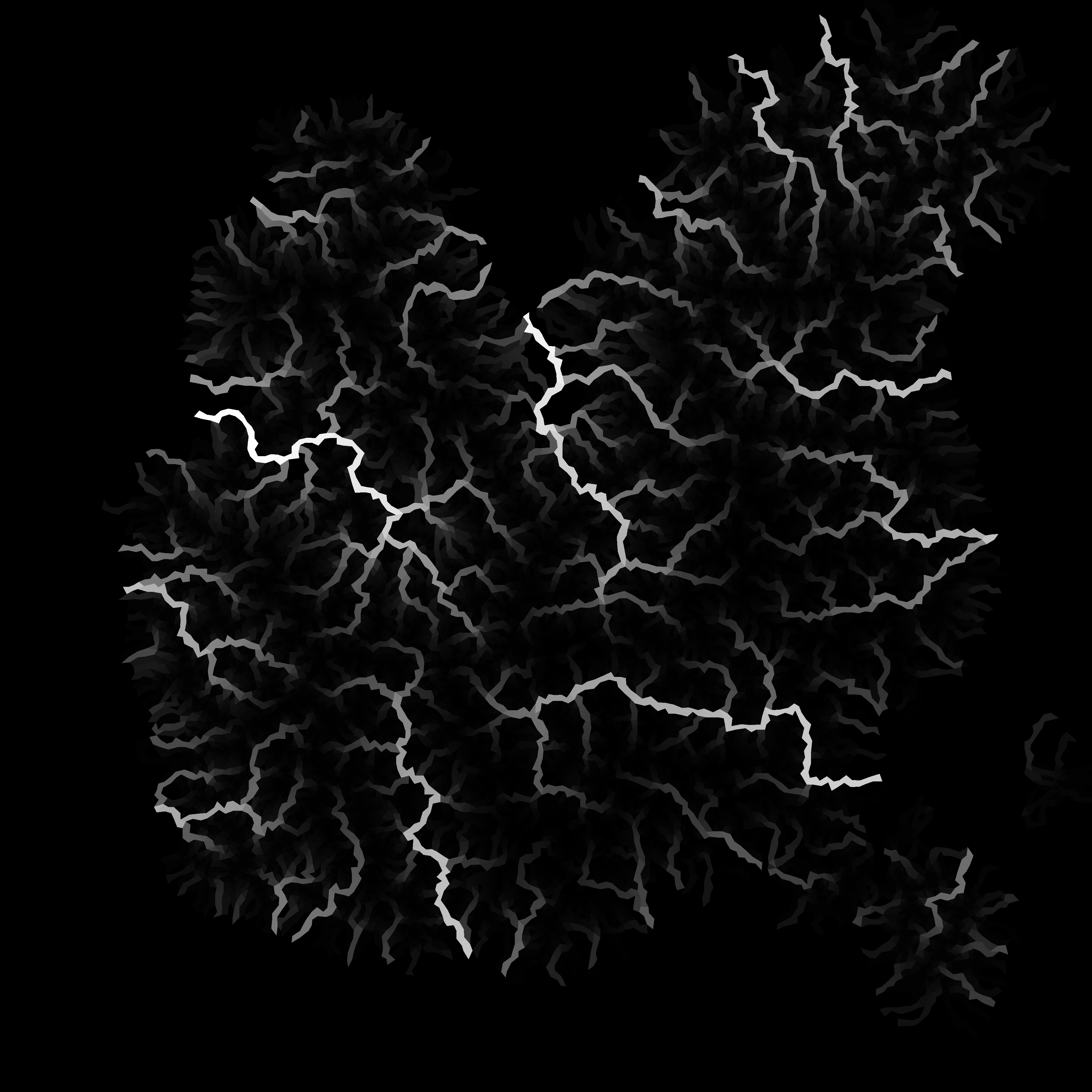
River Flow Accumulation

With slopes assigned, we simulate water flow by accumulating rainfall as it flows downhill:

The Flow Algorithm

assign_flow works on top of the downslope graph produced earlier. We initialise every land triangle’s runoff from its local moisture (flow * moisture²), then walk triangles from the peaks down to the coast using the previously recorded visit order.

for &t_tributary in triangle_order.iter().rev() {
    if let Some(t_trunk) = downstream_triangle(mesh, t_tributary, downslope_s) {
        let flow = triangle_flow[t_tributary];
        triangle_flow[t_trunk] += flow;      // accumulate volume
        halfedge_flow[s_flow]      += flow;  // store river segment flow

        if modified_elevation[t_trunk] > modified_elevation[t_tributary]
            && modified_elevation[t_tributary] >= 0.0
        {
            modified_elevation[t_trunk] = modified_elevation[t_tributary];
        }
    }
}

Because the traversal order already guarantees we see every tributary before its trunk, no priority queue or HashMap is required during accumulation. The companion array halfedge_flow gives us the per-edge flow rate that the viewer visualises.

(downstream_triangle in the snippet is just shorthand for the halfedge/twin lookup present in the code.)

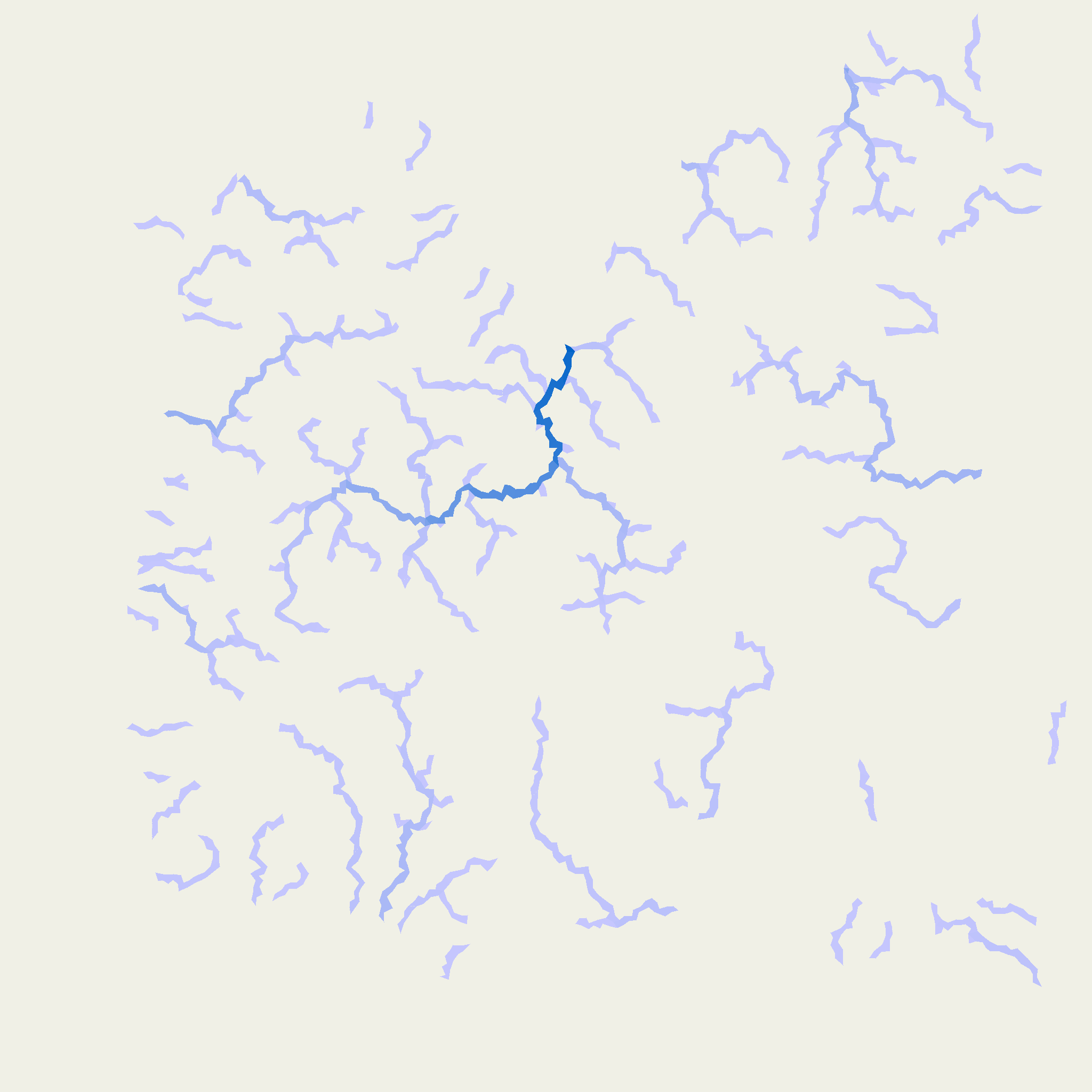
River Rendering

Rivers appear where flow exceeds a threshold. We render them as blue lines with width proportional to flow:

The viewer’s debug renderer reads the accumulated halfedge_flow and draws anti-aliased line segments between triangle centroids. Colour intensity scales with flow volume, and for larger rivers we add a pair of offset strokes to fake extra width. No logarithmic scaling is involved yet—the visual thickness is driven by the raw flow magnitude and capped for stability.

Valley Carving

Rivers don’t just flow over terrain; they carve it. During flow accumulation we opportunistically enforce downhill consistency: whenever a tributary sits above sea level and drains into a taller neighbour, we simply flatten that neighbour to the tributary’s elevation.

if modified_elevation[t_trunk] > modified_elevation[t_tributary]
    && modified_elevation[t_tributary] >= 0.0
{
    modified_elevation[t_trunk] = modified_elevation[t_tributary];
}

It’s a deliberately conservative carve—there’s no logarithmic depth, ridge-distance falloff, or post-processing smoothing yet—but it guarantees the final triangulation respects downhill flow without erasing coastlines.

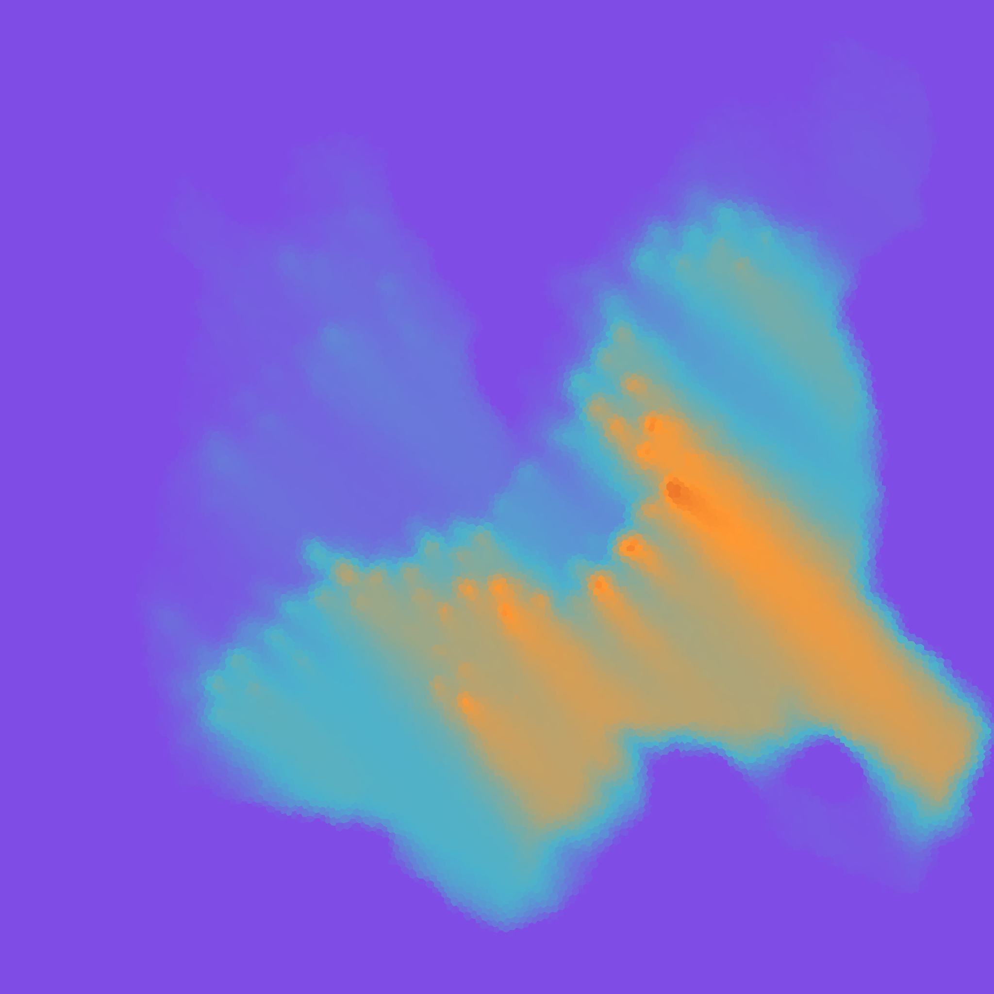
Moisture Calculation

Triangle moisture is simply the average of the rainfall at its three corners. This keeps moisture tightly coupled to the wind-and-orographic model and avoids extra passes:

let triangle_moisture = assign_moisture(&delaunay_mesh, &region_rainfall);

We do not yet boost moisture near rivers, so lush riparian corridors are driven indirectly by higher rainfall wherever drainage concentrates.

Drainage Basins & Lakes

Watershed labelling and depression filling are still on the roadmap. Because every triangle currently has a downslope path to the ocean, interior lakes only appear where the base terrain already created them. Future work will revisit the downslope assignment to allow persistent sinks and to flood depressions up to their spill points.

Visual Results

The complete hydrological system creates compelling, realistic terrain:

River Networks

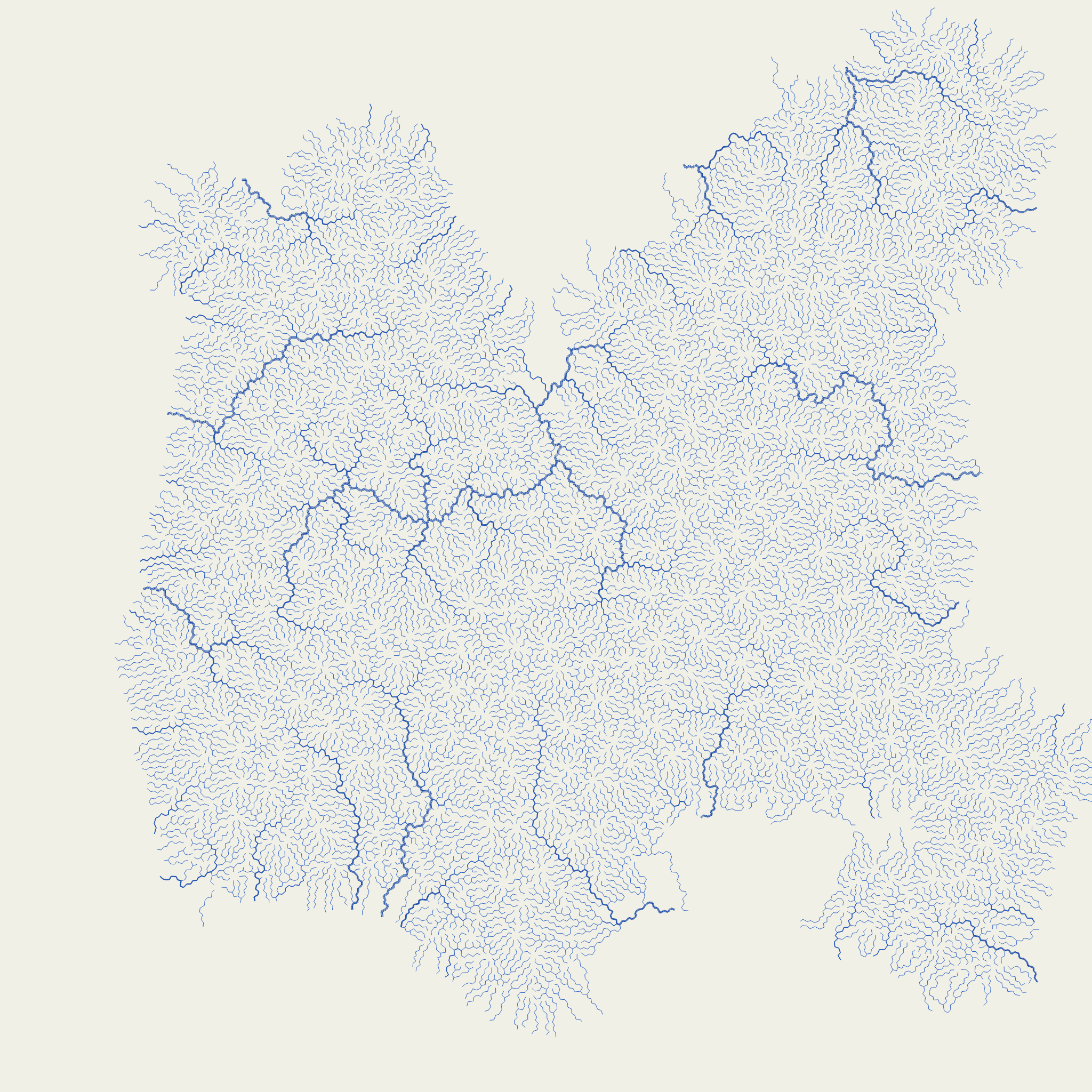
Natural branching patterns emerge from the flow accumulation algorithm.

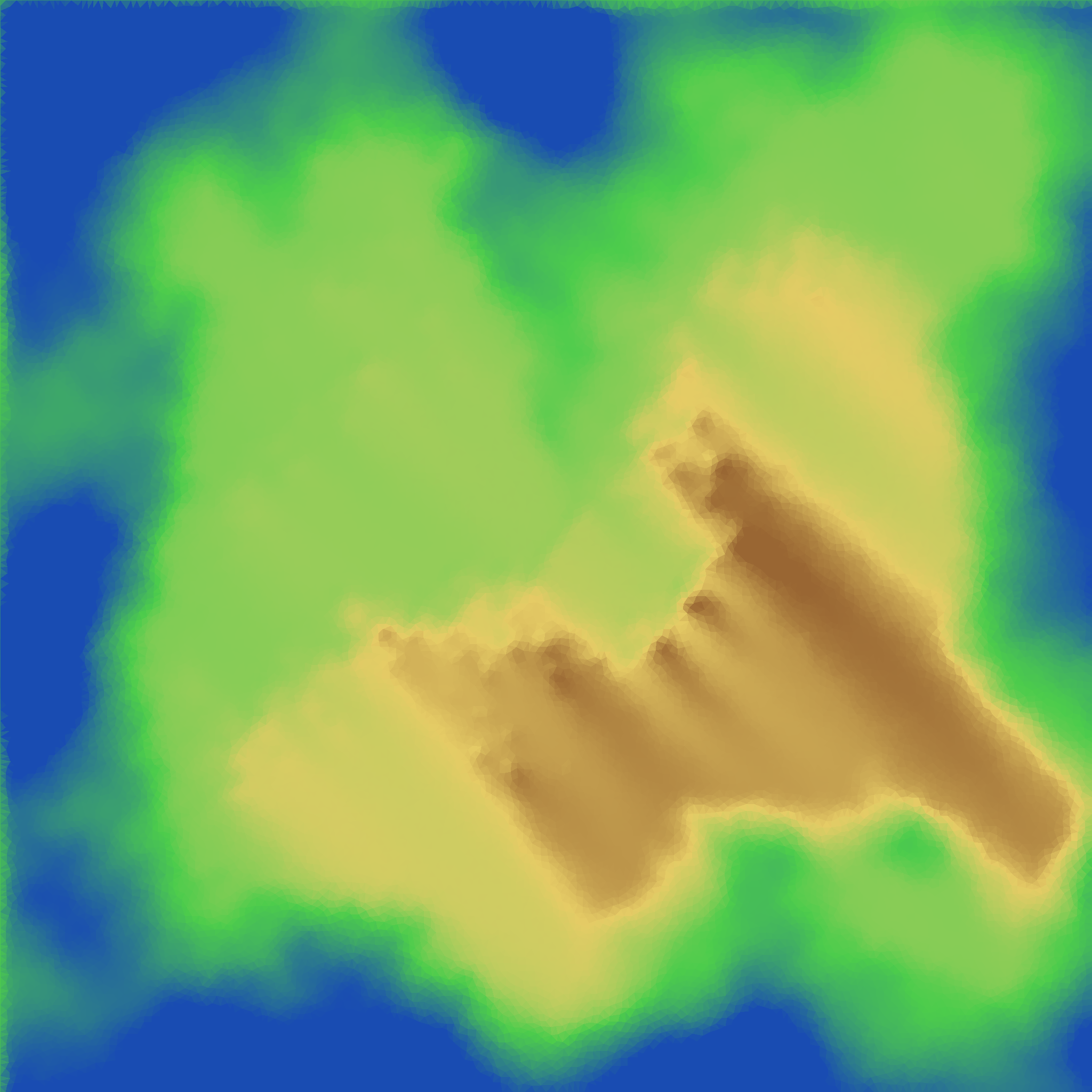
Valley Systems

Rivers carve distinctive valleys while preserving ridge lines.

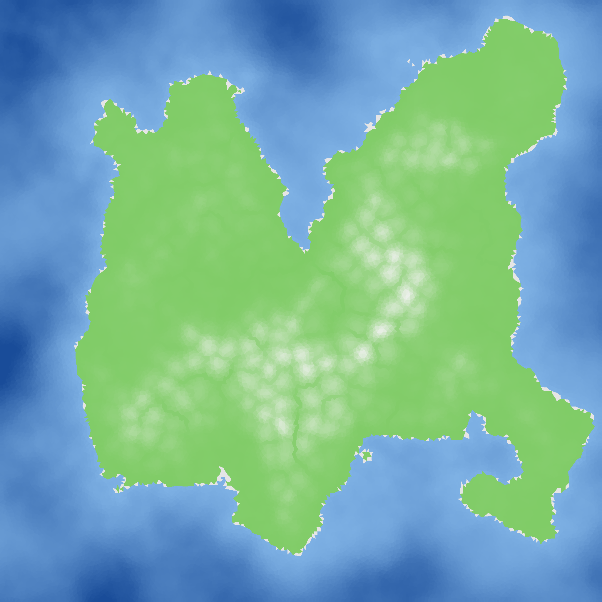
Moisture Patterns

Moisture gradients create natural transitions between biomes.

Mathematical Validation

Two invariants keep the system stable:

1. Directed flow graph – every triangle inherits a downslope edge that eventually reaches the ocean, so accumulated flow is monotonic and non-negative. There are no dangling sources once the ocean seed step completes.
2. Non-invasive carving – valley carving only ever lowers a downstream triangle to match a higher tributary that is still above sea level. Coastlines and underwater regions therefore remain untouched, preventing the algorithm from flooding the island accidentally.

While the current runoff model uses heuristic scaling (flow * moisture²) rather than strict water balance, these constraints keep drainage visually coherent and numerically well-behaved.

Next Steps

With water shaping our landscape, we’re ready to paint it with life. Part V will explore biome generation: how elevation, moisture, and temperature combine to create forests, deserts, tundra, and everything in between. We’ll see how the hydrological system we’ve built drives vegetation patterns and ecosystem boundaries.

The rivers we’ve carved don’t just shape terrain; they define where forests thrive, where deserts form, and where civilizations might emerge.

Valuable Resources

• Hydraulic Erosion - Implementation details
• Stream Power Erosion - Geological background
• Drainage Basin Analysis - Amit Patel’s watershed algorithms