Procedural Island Generation (V)
This post is a direct continuation to Part IV, where we simulated the hydrological cycle. Now we’ll paint our island with life, using elevation and moisture to generate realistic biome distributions.
Biomes emerge from the interplay of climate factors. Temperature drops with altitude, moisture varies with rainfall and proximity to water, and these gradients create distinct ecological zones. CartoKit distils that idea into two ingredients—elevation and moisture—and uses them to drive both a continuous colour ramp and a handful of coarse biome tags.
Biome Buckets
CartoKit takes a deliberately small-step approach to biome classification. The exporter stores a coarse BiomeType per triangle so downstream tools can switch materials or spawn vegetation without re-running the full generator. The thresholds live inside Terrain::classify_biome (src/terrain.rs:683):
fn classify_biome(elevation: f32, moisture: f32) -> BiomeType {
    if elevation < -0.5 {
        BiomeType::DeepOcean
    } else if elevation < 0.0 {
        BiomeType::ShallowOcean
    } else if elevation < 0.01 {
        BiomeType::Beach
    } else if elevation < 0.3 {
        if moisture < 0.3 {
            BiomeType::Desert
        } else if moisture < 0.6 {
            BiomeType::Grassland
        } else {
            BiomeType::Forest
        }
    } else if elevation < 0.6 {
        if moisture < 0.33 {
            BiomeType::Tundra
        } else {
            BiomeType::Taiga
        }
    } else {
        BiomeType::Snow
    }
}
That yields the following buckets:
| Elevation band | Moisture split | BiomeType |
|---|---|---|
< -0.5 |
— | Deep Ocean |
[-0.5, 0) |
— | Shallow Ocean |
[0, 0.01) |
— | Beach |
[0.01, 0.3) |
<0.3 Desert / [0.3,0.6) Grassland / ≥0.6 Forest |
|
[0.3, 0.6) |
<0.33 Tundra / ≥0.33 Taiga |
|
≥0.6 |
— | Snow |
It is intentionally conservative: we only need enough variety to drive material swaps and the color ramp; anything more granular is left to future work.
Continuous Color Mapping
Visuals are driven by a continuous color function instead of discrete textures. The public API exposes calculate_biome_color (src/biome.rs:15), which maps elevation ∈ [-1,1] and moisture ∈ [0,1] to an RGBA value:
pub fn calculate_biome_color(elevation: f32, moisture: f32) -> [u8; 4] {
    let mut m = moisture.clamp(0.0, 1.0);
    let e = elevation.clamp(-1.0, 1.0);

    if e < 0.0 {
        let r = (48.0 + 48.0 * e).max(0.0) as u8;
        let g = (64.0 + 64.0 * e).max(0.0) as u8;
        let b = (127.0 + 127.0 * e).max(0.0) as u8;
        [r, g, b, 255]
    } else {
        m *= 1.0 - e;
        let base_r = 210.0 - 100.0 * m;
        let base_g = 185.0 - 45.0 * m;
        let base_b = 139.0 - 45.0 * m;

        let r = (255.0 * e + base_r * (1.0 - e)).min(255.0) as u8;
        let g = (255.0 * e + base_g * (1.0 - e)).min(255.0) as u8;
        let b = (255.0 * e + base_b * (1.0 - e)).min(255.0) as u8;
        [r, g, b, 255]
    }
}
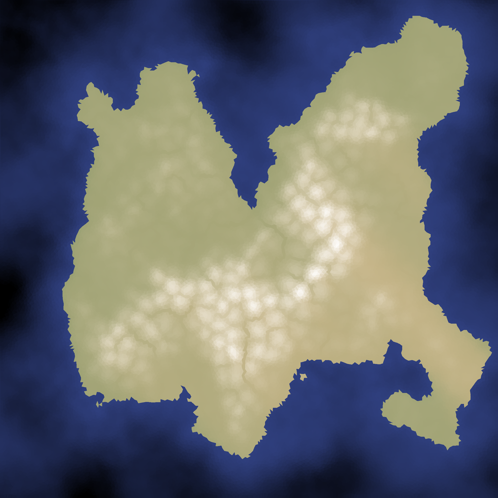
- Oceans fade from deep blue to turquoise as depth decreases.
- Land blends tan through green based on moisture, then ramps toward white as elevation climbs.
Because the function is continuous, neighbouring triangles share smooth colour transitions without an explicit blending pass.
2D Colormap Visualisation
The viewer’s “Biome Colormap” debug mode is powered by debug::biome_colormap::generate_colormap (src/debug/biome_colormap.rs:22). It bakes the function above into a 2D texture where the X-axis is elevation and the Y-axis is moisture, letting us inspect the palette or export it for documentation.
let params = ColormapParams::default();
let image = generate_colormap(¶ms);

Viewer Rendering
In the interactive viewer, the Biome and BiomeWithRivers display modes simply evaluate calculate_biome_color per triangle. The river overlay multiplies river flow onto the colour buffer so wet channels read clearly against the base biome ramp. There is no seasonal tinting, riparian override, or microclimate logic yet—those panels in the UI are placeholders for future experiments.

Exported Attributes
When we bake a Terrain, every face stores:
- Average elevation and moisture (from vertex attributes).
TerrainType(land vs water) and the coarseBiomeTypebucket fromclassify_biome.
This information is embedded alongside the final triangulation mesh so external tools can colour-code or spawn assets without re-running CartoKit.
Performance Notes
Biome work piggybacks on data we already track:
| Operation | Time (27K triangles) |
|---|---|
calculate_biome_color sampling in viewer |
~1 ms |
classify_biome during export |
~1 ms |
| Colormap bake (64×64) | ~1 ms |
The runtime cost is negligible compared to hydrology—the colour ramp is just a handful of arithmetic ops per triangle.
Future Improvements
Several ideas from early design notes (temperature lapse rates, seasonal palettes, riparian upgrades, succession) have not been implemented yet. If we revisit biomes in the future, that backlog will drive the next iteration. For now the focus stays on delivering a stable colour ramp and a compact set of biome tags that downstream tools can consume reliably.
Next Steps
Our island now pulses with life, painted in the colors of its ecosystems. Part VI, the final installment, dives into the baked Terrain output, the egui viewer, and the GLB/PNG/GIF export helpers that ship the result.
From the mathematical foundations to the living landscape, we’ve built a complete procedural island generation system. The conclusion awaits.
Valuable Resources
- Whittaker’s Biome Classification - Original biome model
- Vegetation Procedural Generation - Red Blob Games biome techniques
- Ecotones and Edge Effects - Transition zone ecology