Growing trees
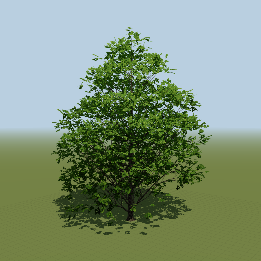
I’ve been playing with procedural tree growth recently. The method I am using is based on Self-organizing tree models for image synthesis, by Palubicki et al. (SIGGRAPH 2009).
The idea is beautifully simple: buds compete for light, the tree distributes a growth resource among them, and the successful ones produce new shoots. Those shoots change the light available for the next round. The crown shape emerges from this feedback loop.
Here is a quick breakdown, with some visualizations from my implementation.
One season at a time
The basic building block is a metamer: an internode (a short piece of stem), a leaf, and the buds at its upper node. A terminal bud continues an axis, and axillary buds may start lateral branches.
Each iteration represents one growing season:
- Measure the light available to every bud.
- Sum that light from the tips down to the root.
- Distribute a proportional growth resource back up the tree.
- Grow shoots from the buds that receive enough resource.
- Shed poorly lit branches and age dormant buds.
Where is the light?
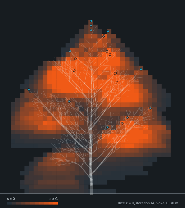
One way to approximate light availability is a voxel grid. Each bud adds shadow to a widening pyramid of voxels below it, with its contribution decaying with depth. Contributions from all buds add up, so the interior naturally becomes darker as the tree grows.
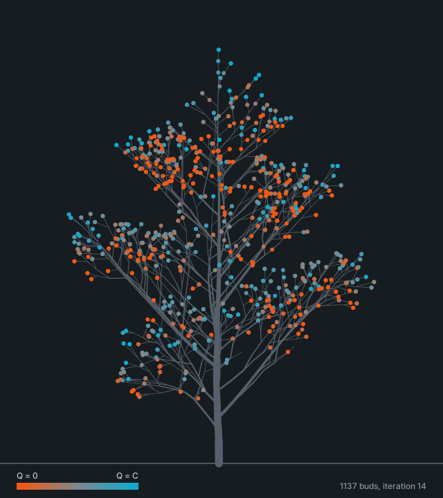
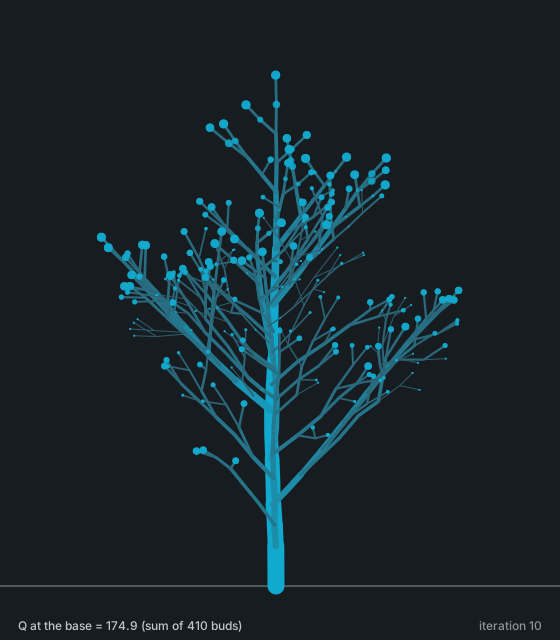
Each bud reads two things from this grid: an available-light value \(Q\), and a direction \(\mathbf{V}\) toward the least shaded neighboring voxel inside its perception cone.
The paper also supports space colonization: fill an envelope with marker points, let buds compete for nearby markers, and remove markers as growth occupies their space. Same growth machinery, a different way to decide where growth is possible.
Who gets to grow?
Light values are first summed down the branching structure. At the base, the total \(Q_{base}\) becomes a growth resource \(v=\alpha Q_{base}\). This resource travels back up, splitting at every branching point.
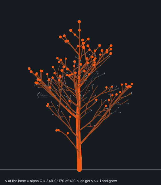
In the extended Borchert-Honda model, the main continuation receives:
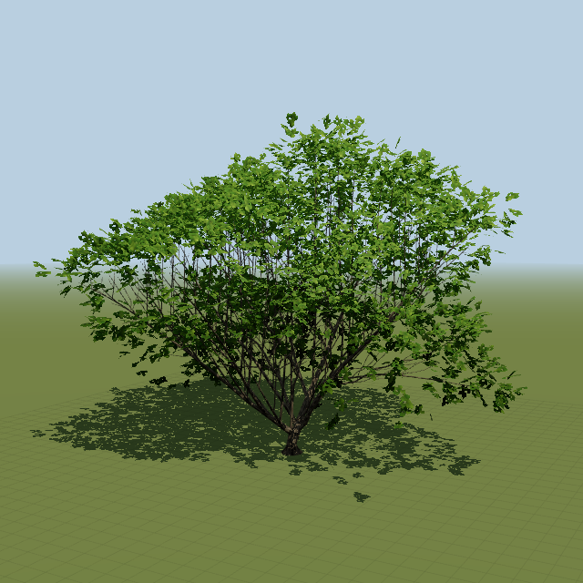
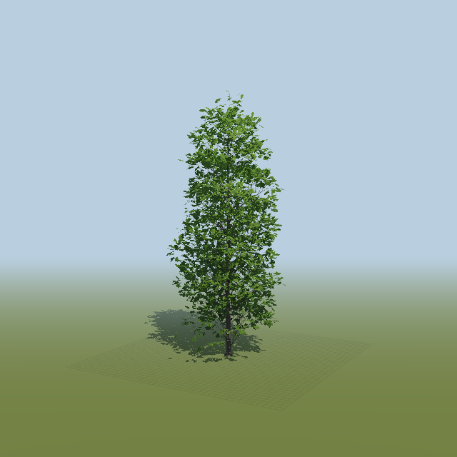
\[v_m=v\frac{\lambda Q_m}{\lambda Q_m+(1-\lambda)Q_l}\]The lateral side receives the remainder. At \(\lambda=0.5\), resource follows light. Larger values favor the main axis. Smaller values favor the laterals.
This little bias has a surprisingly large effect:
A bud receiving less than one unit stays dormant. Otherwise it produces a shoot of \(\lfloor v\rfloor\) metamers, subject to a configured cap. New metamers receive their own buds, and the process repeats. Magic!
Which way?
Each new segment follows a normalized weighted sum of its previous direction, the light-seeking direction \(\mathbf{V}\), an upward or downward tropism, and some noise. A horizontal component can make lateral branches spread into flat tiers.
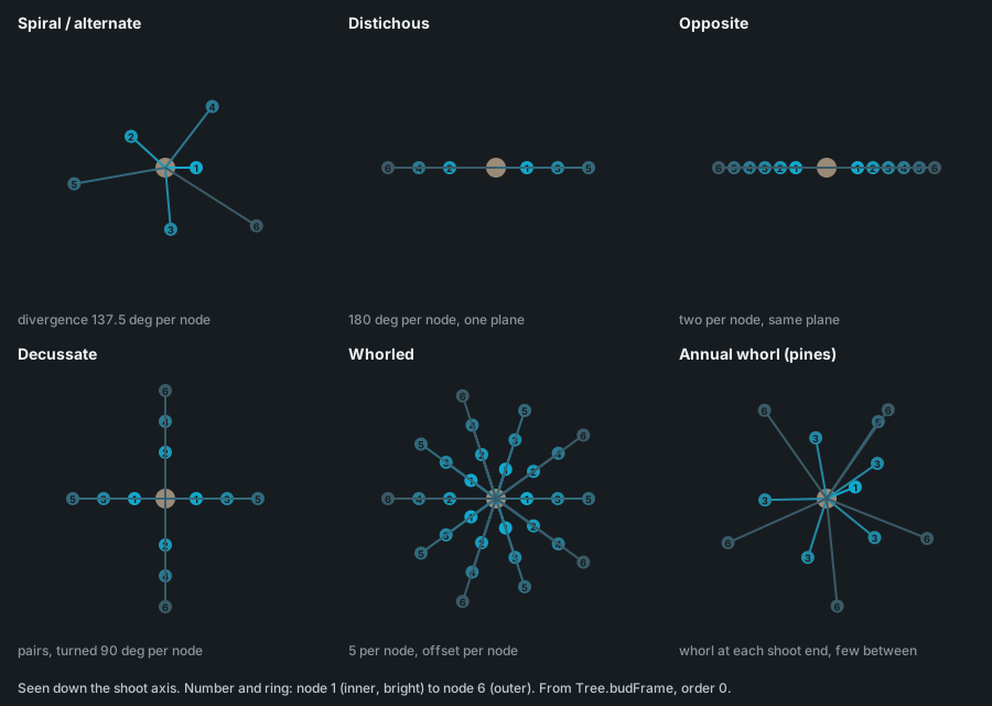
Bud placement around the stem (phyllotaxis) provides another important control. Spiral arrangements, opposite pairs, and annual whorls produce very different branching patterns. The frame is parallel-transported along the shoot so the arrangement stays coherent as it bends.
Dropping branches and adding girth
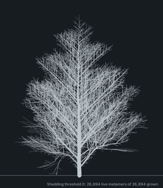
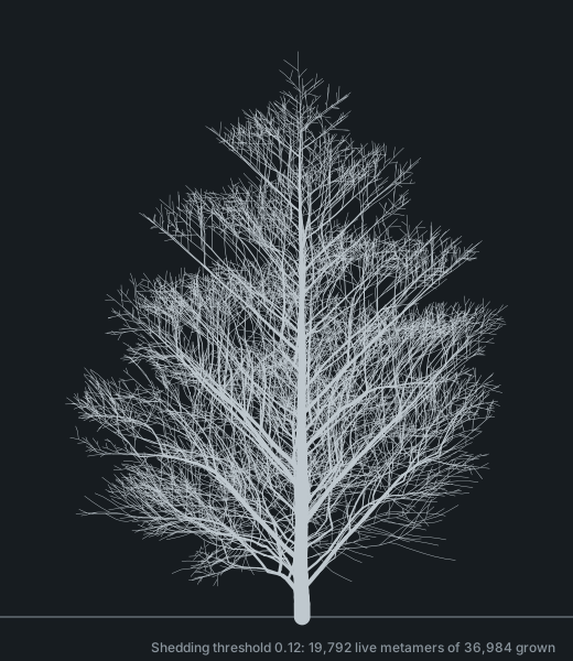
With the shadow model, a lateral branch is shed when the light collected by its subtree, divided by its metamer count, falls below a threshold. Young branches get a grace period. Otherwise the inner crown would keep accumulating starved twigs.
Branch thickness comes afterwards, using a pipe model:
\[r_{parent}^{n}=\sum_i r_i^{n}\]Start with a fixed radius at the tips and accumulate toward the root. For \(n=2\), cross-sectional area is preserved at junctions. Larger exponents produce slenderer trunks. Shed branches still contribute to the girth below them. Losing a branch does not make the trunk shrink.
Width and passive sag are calculated from the grown skeleton and do not feed back into growth.
From branches to foliage
The skeleton becomes a bark mesh by sweeping tubes along its axes. For foliage I use twig spray cards: each card depicts a small twig carrying several leaves, using variants from a procedurally drawn atlas.
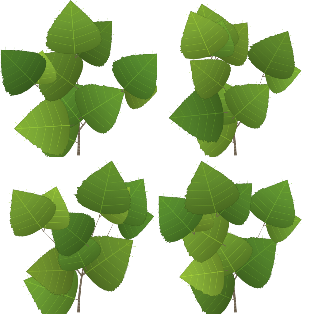
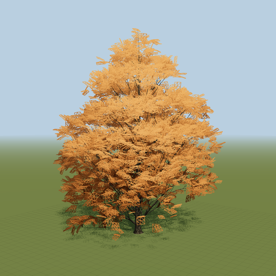
Blending the card normals toward an ellipsoid around the crown helps the foliage shade as a volume. Lower detail levels retain fewer, larger cards and simplify the bark. At a distance, baked directional impostors take over.
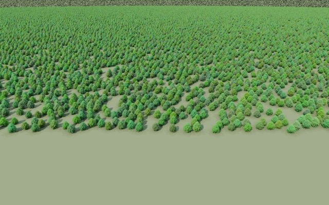
Bonus: The grown tree can also be baked into depth-field views for forest rendering. The image below uses many instances of one baked linden, with size variation. The forest representation and lighting deserve a separate post, though.