Truncated SVD

PCA

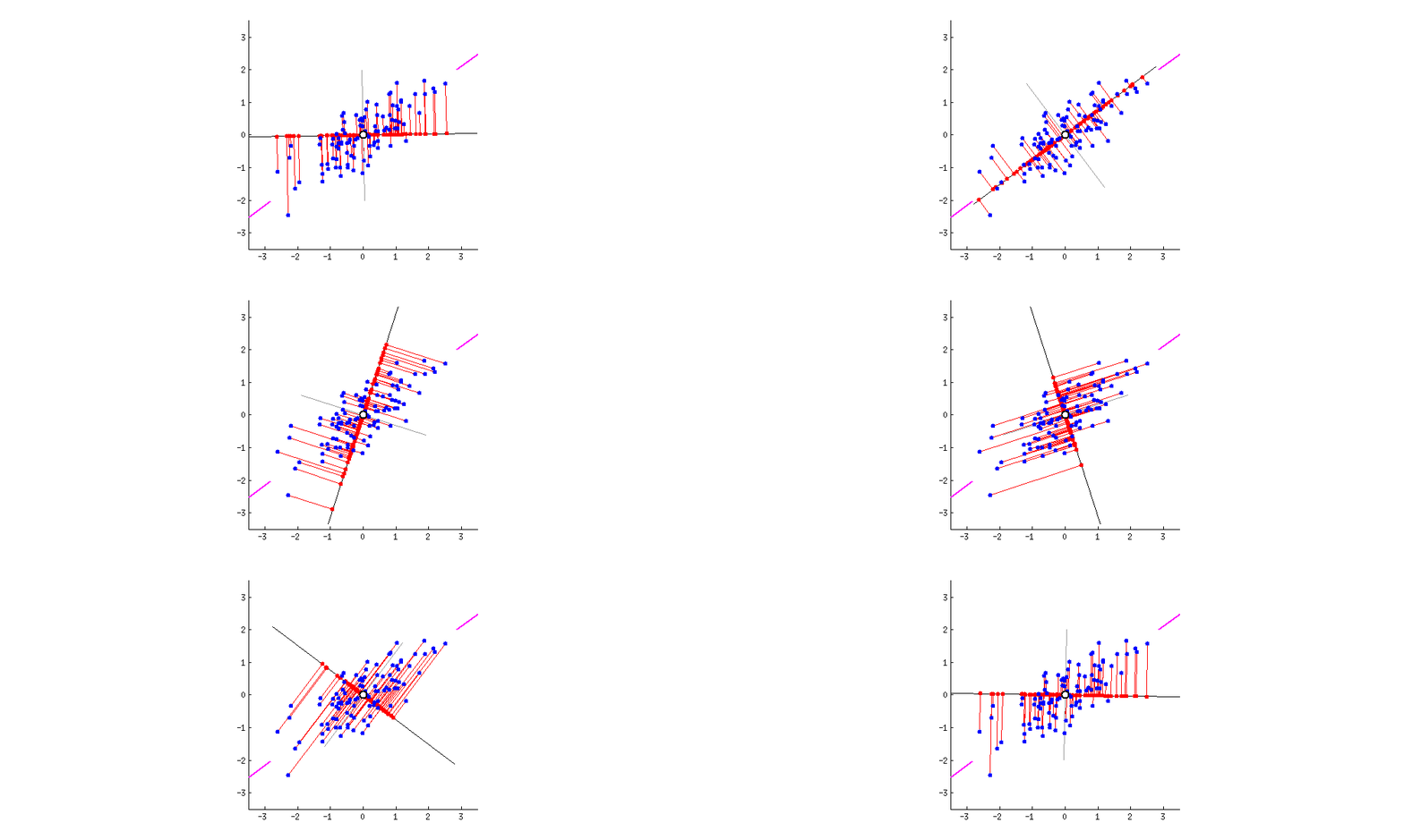
Principal Component Analysis (PCA) is the subject of a previous post of mine, so I will only summarize it here.

Data reduction via PCA is accomplished by linearly transforming the data into a new coordinate system where (most of) the variation in the data can be described with fewer dimensions than the initial data.

Without getting into the details, this involves an eigen-decomposition of the covariance matrix.

SVD

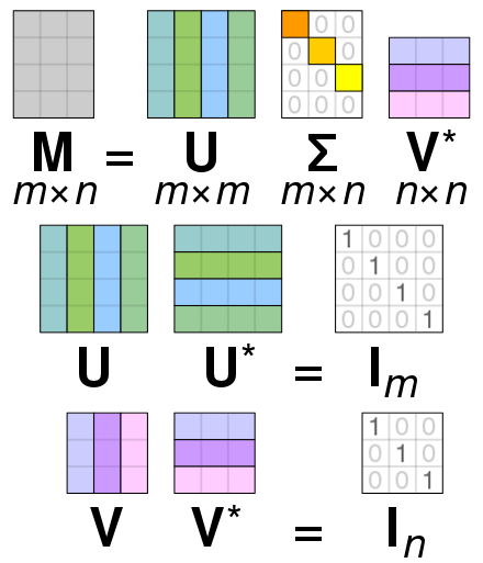
Singular Value Decomposition (SVD) is a matrix factorization technique that factors a real matrix M into three matrices U, Σ, and V such that M=U*Σ*V^T.

If M is mxn, then U is mxm, Σ is mxn and V is nxn. Both U and V are orthonormal, and Σ is rectangular-diagonal with non-negative coefficients.

This is very similar to PCA, excepting that the factorization for SVD is done on the data matrix, whereas for PCA, the factorization is done on the covariance matrix.

The diagonal coefficients of Σ are known as the singular values of M and it is common practice to rearrange the SVD so the singular values are given in decreasing order. The number of non-zero singular values is equal to the rank of M.

The SVD is tightly related to PCA:

• The columns of V are principal directions/axes (eigenvectors).
• Columns of U*Σ are principal components (scores).
• Singular values are related to the eigenvalues of the covariance matrix.

From Wikipedia:

Truncated SVD

Let’s try with a 1024x1024 grayscale image of the moon:

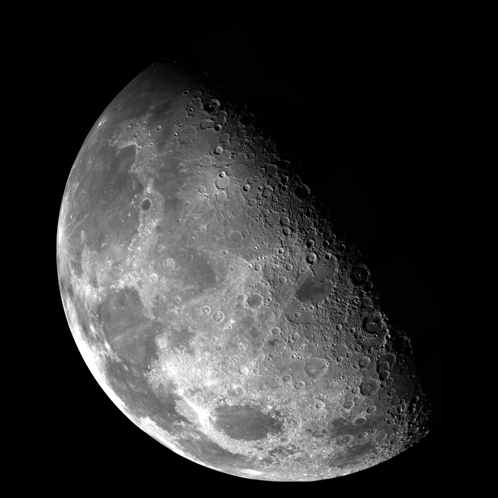
Such an image can be interpreted as 1024 vectors of 1024 components each. i.e., a set of 1024 vectors in a 1024-dimension space.

If we run PCA/SVD on this set, the three matrices U, Σ, V will be 1024x1024. In particular, Σ will be a square-diagonal matrix. i.e., only the coefficients in the diagonal are potentially non-zero. It is common practice to rearrange the three matrices so the diagonal indices in Σ are sorted from greater (top-left) to lower (bottom-right).

Truncated SVD is simply the act of zeroing-out all the coefficients in Σ except for the top-left n ones.

Coefficient truncation implies that we’re also trashing 1024-n columns in U and in V (as now those will be multiplied by 0 anyway).

If we now reconstruct the original matrix M'=U'*Σ'*V'^T using the truncated matrices, we will obtain M', which will resemble M. The fewer the coefficients that we drop, the more closely that M' will approximate M. But because of the information-preserving properties of PCA/SVD, keeping just a bunch of the topmost coefficients in Σ may suffice to restore all (or near all) the original information.

Reconstructing the moon

Let’s put all of the above to work on the moon image. Truncating at a single value of n is not particularly illustrative, so instead we will sweep n across its whole range and watch how the approximation behaves.

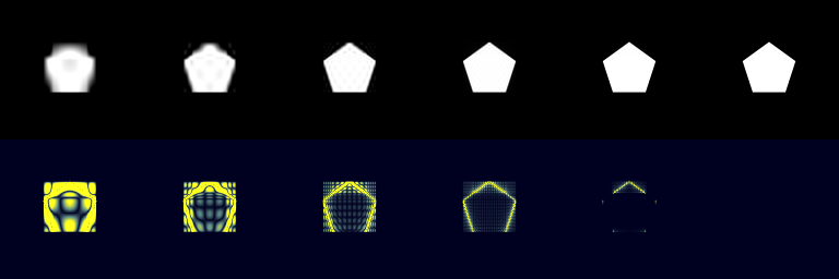
The images and videos that follow all share the same layout:

• The left half is the reconstructed matrix M'.
• The right half is the reconstruction error abs(M-M').
• The decreasing yellow graph is the MSE as fewer and fewer singular values are zeroed-out.

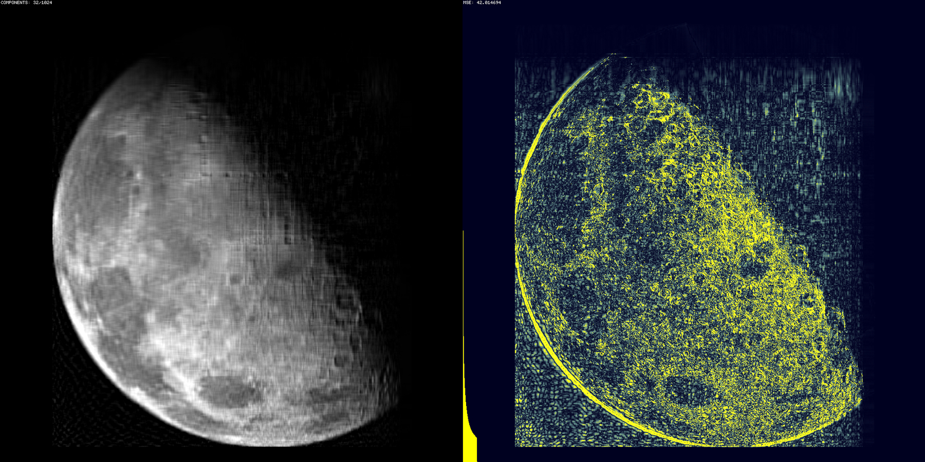
This screenshot is M' reconstructed with only 32 (out of 1024) components. Right click + Open in new tab for 1:1 quality.

It is worth pausing on what those 32 components actually cost us. The truncated factors are U' (1024x32), the 32 surviving singular values, and V' (1024x32). That is 65568 numbers, versus the 1048576 numbers in M. i.e., a 16x reduction, for an image that still reads as the moon.

Below is a video with the same image pair as more and more components are used for reconstruction. Most of the action happens in the first few frames.

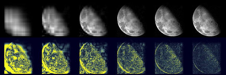
What’s remarkable here (the magic of PCA/SVD) is how quickly the error graph decreases. This proves that the first components capture most of the information present in M, while the trailing components only carry high-frequency/low-amplitude fine details.

This is reminiscent of what happens with the Fourier Transform, the Cosine/Sine Transform and such. Those transforms deal with the space vs. frequency duality, whereas PCA/SVD is purely a variance-driven change-of-basis. But in a similar fashion, all these methods transform information to a dual form where the “amount of information” emerges in a structured, manageable way.

The FT/CT/etc… lie at the foundation of .jpeg, .mp3 and other compression systems which exploit the fact that the Human Perception System is more sensitive to luminance (vs. chromaticity), and to lower (vs. higher) frequencies.

In the case of SVD/PCA, the upper coefficients in Σ capture more data variance than the lower ones.

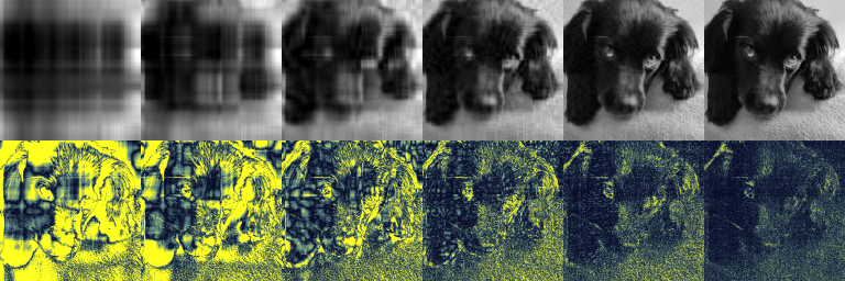
These sequences are reconstructions with 2, 4, 8, 16, 32, 64, and 128 coefficients.

Easier vs. harder cases

As explained above, the matrix factorization can be interpreted as a change of basis to a special space where the data has rows which are linearly dependent with each other. In such case, U/V matrices of a lower rank will suffice to reconstruct the original matrix exactly. Actually, Σ will present itself with as many zero-valued coefficients in its diagonal as rows/columns can be trashed without causing any loss of data.

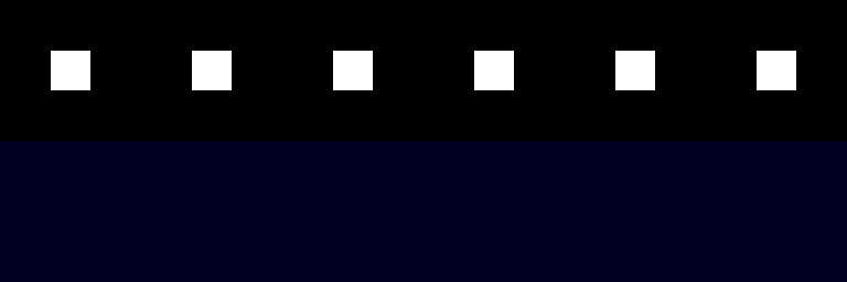
An extreme case is presented below (a centered square box shape), where 1 coefficient/row/col suffices. In this case both inside and outside the shape, all rows/cols are identical. A box is a separable convolution filter, BTW (future post on low-rank convolution incoming, I hope).

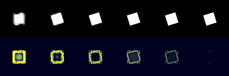
Rotating the shape brings disaster even though PCA/SVD are capable of “auto-detecting” such changes of basis. But here we’re dealing with discrete math, so the rotated shape gets “pixelated” and this makes the decomposition become numerically impure.

It’s funny to see how in the first frames of the video the reconstruction “insists” on being an unrotated square, somehow.

Below, a pentagonal shape.

Practical uses

There are interesting practical uses for SVD truncation other than dimensionality reduction in data analysis.

Data compression

Bart Wronski has a very interesting write up on compression of PBR texture sets using this technique.

BCn Texture Compression is based on dimensionality reduction as well. Nice write up on the subject by Nathan Reed.

Low-rank approximation

Low-rank approximation.

Another interesting read by Bart Wronski. I wish to do my own write up on low-rank convolution at some point.

Implementation details

I had some old PCA/SVD C++ code in Maverick’s API, which I used for the images/videos in this post. But after reading this post by Atrix256 I may bite the bullet and replace the implementation part of my old xsvd_c class with Eigen.