Procedural Island Generation (III)
This post continues from Part II, where we established the paint map foundation and mountain ridge system. Now we’ll add detailed noise layers, distance-based mountain peaks, and do blending to create the final terrain elevation.
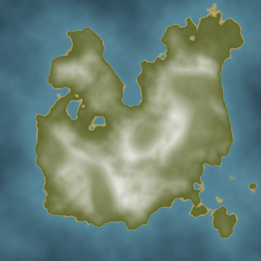
Paint Map (recap)
Before applying noise layers, we start with the foundation established in Part I - the paint map that defines our base land/water distribution:
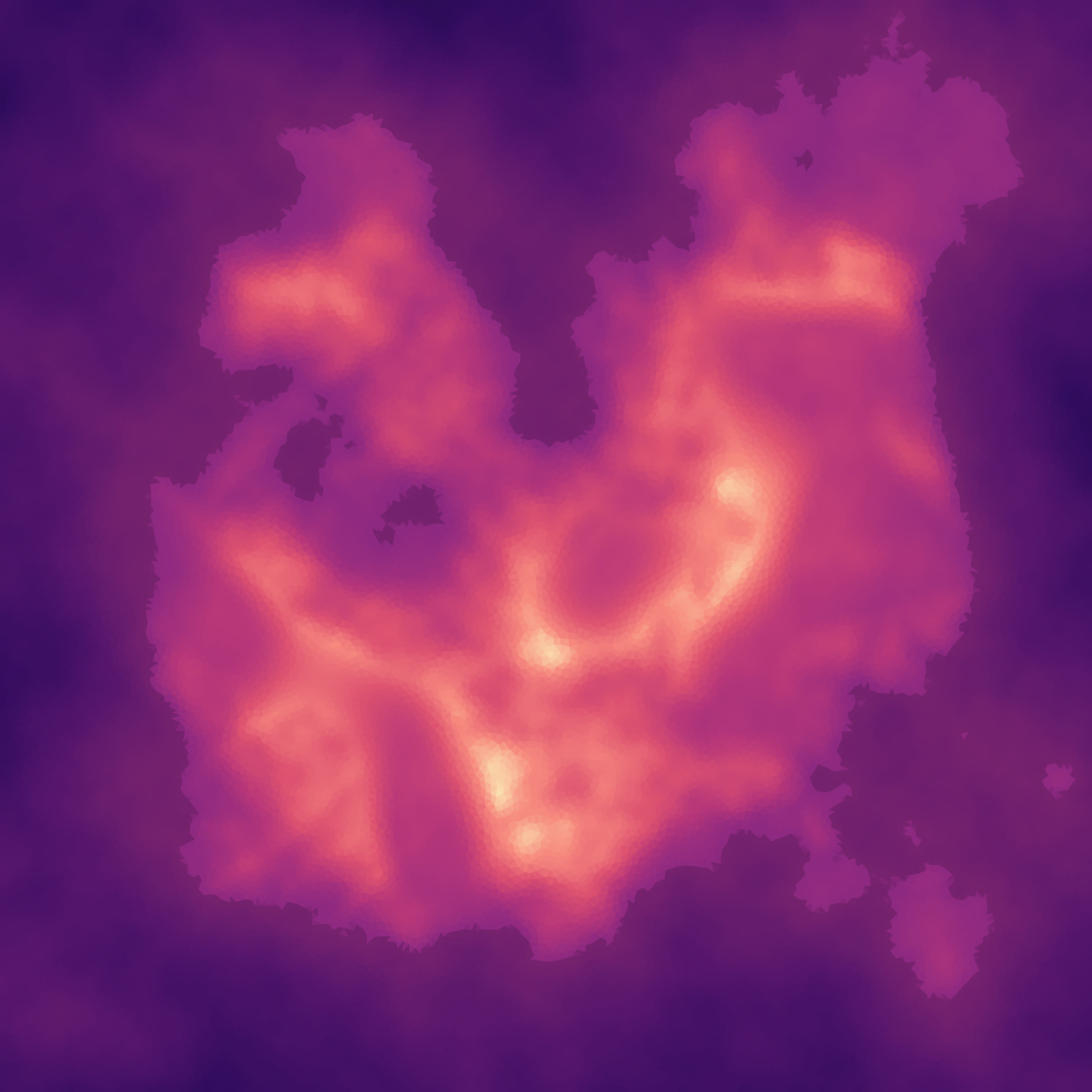
For visualization throughout this post, we’ll be using the magma palette from matplotlib, which I patched to artificially darken the ocean areas to highlight the coastline:
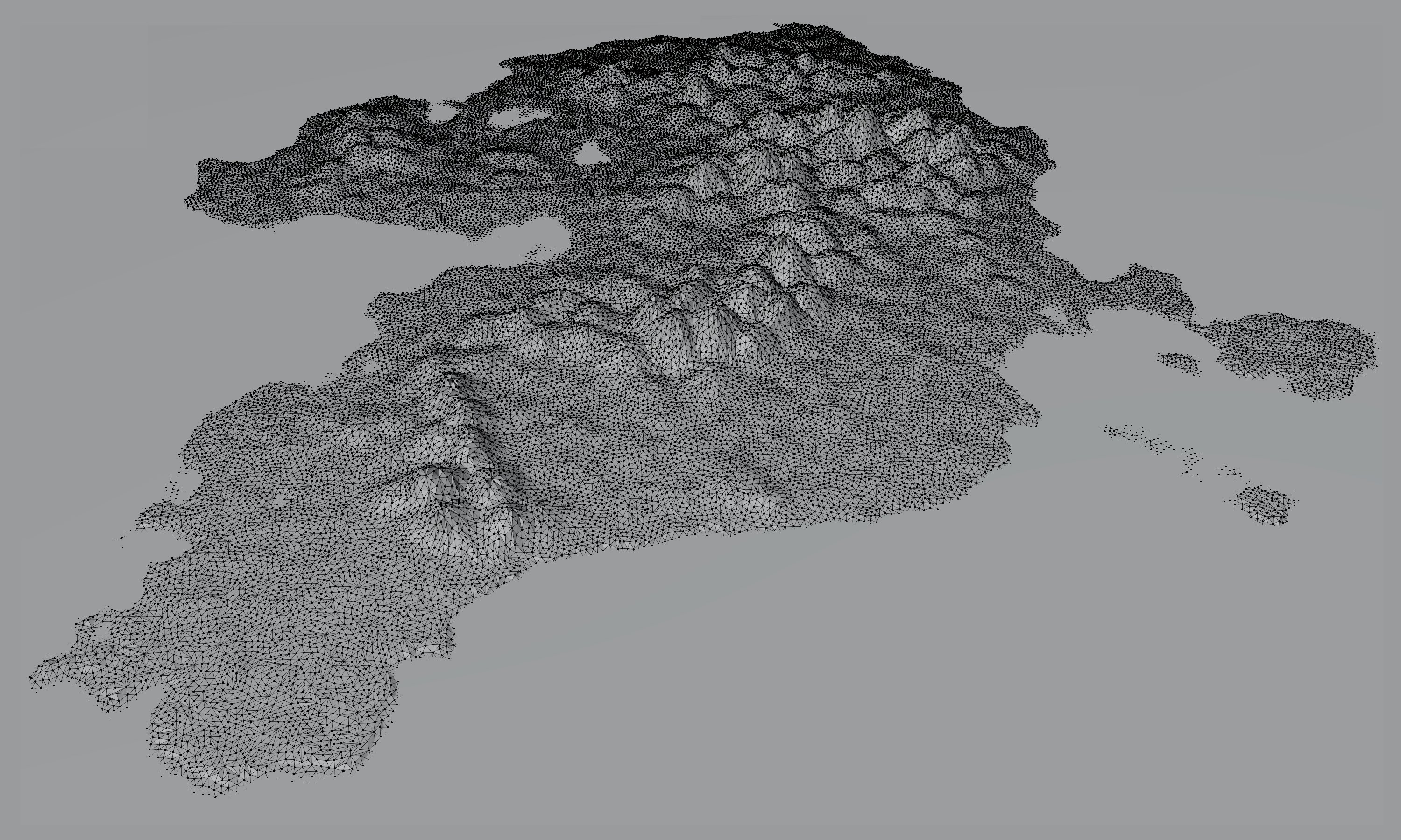
Note that we’ll be sampling the paint map per Delaunay triangle (at each triangle’s centroid):

Remember that the paint map provides the broad strokes: positive values for land, negative for ocean, with smooth transitions between them. Now we’ll enhance it with noise layers to create realistic terrain detail.
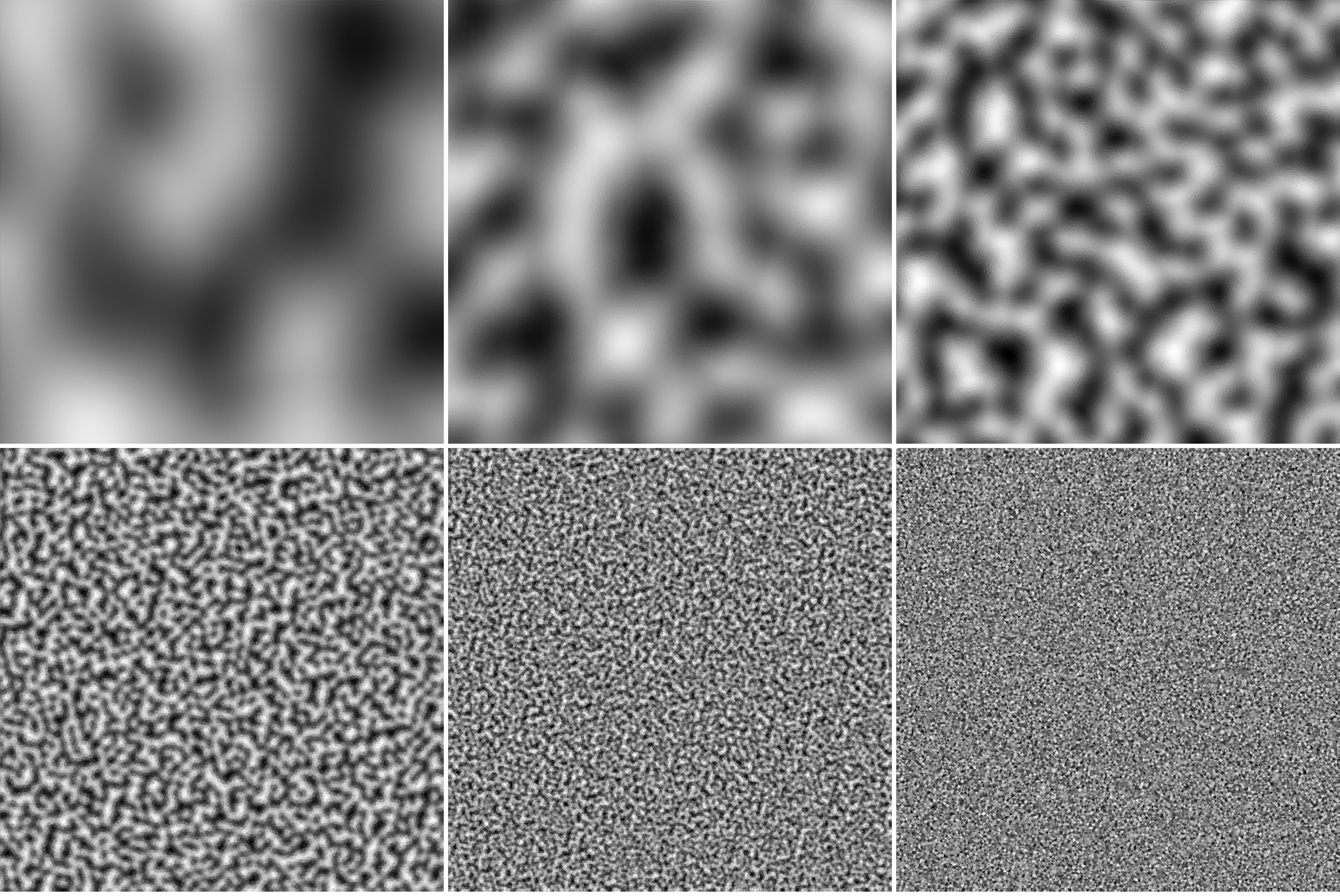
Multi-Scale Noise Layers
We will layer multiple octaves of Simplex noise at different frequencies over the broad strokes provided by the paint map. Each will contribute different detail scales to the final terrain.
mapgen4 by @redblobgames in particular uses six layers:
| Layer | Frequency | Description |
|---|---|---|
| n₀ | 1x | Lowest frequency |
| n₁ | 2x | Low frequency |
| n₂ | 4x | Medium-low frequency |
| n₄ | 16x | Medium-high frequency |
| n₅ | 32x | High frequency |
| n₆ | 64x | Highest frequency |
Notice the gap in numbering (n₃ is missing). This would correspond to frequency 8x, which we don’t use.
Coastal Noise Enhancement
mapgen4 starts with coastal noise enhancement. This provides control over the variation at coastlines while keeping inland elevation unaffected:
\[e = \text{Paint map from Part I}\] \[e_{coast} = e + \alpha \cdot (1 - e^4) \cdot \left(n_4 + \frac{n_5}{2} + \frac{n_6}{4}\right)\]The term \((1 - e^4)\) creates a bell curve that peaks at \(e=0\) (coastline) and decreases rapidly for \(\lvert e \rvert > 0\). This modulates an fBm-like combination of our three highest frequency noise layers.
What matters here isn’t the exact formula or amplitudes, but the core principle: applying high-frequency detail specifically where land meets water.
\[e_{tmp} = \begin{cases} e & \text{if } e_{coast} > 0 \\ e_{coast} & \text{if } e_{coast} \leq 0 \end{cases}\]Mountain Distance Field
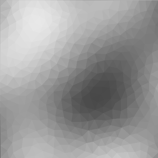
Mountains need special pre-processing. If you remember from Part I in the swarm of seed points we tagged some as mountain peaks. Here we will pre-compute a distance field from every regular seed point to the closest mountain peak point.
We compute distance through the mesh topology of the Delaunay triangulation using BFS (breadth-first search). i.e., we don’t use Euclidean distance. This creates more organic mountain shapes that follow the terrain’s natural connectivity.
The algorithm spreads outward from mountain peaks:
- Start at triangles containing mountain seed points (distance = 0)
- Visit neighboring triangles, incrementing distance by a randomized amount
- The randomization creates natural ridge patterns instead of perfect cones
Here’s the magic formula used for distance increment in each step:
\[\Delta = s \cdot (1 + j \cdot r)\]Where:
- \(s\) = spacing between triangles (uses configured Poisson disk separation)
- \(j\) = jaggedness parameter (0 = true topological distance, 1 = very irregular)
- \(r \in [-1,1]\) = random factor using triangular distribution
The triangular distribution rand() - rand() clusters values near zero while allowing occasional larger variations. This looks more natural than uniform randomness.
I implemented Fisher-Yates shuffling when visiting neighbor triangles. Instead of processing neighbors in a fixed order (which would create directional bias), the order is randomly shuffled each time. This ensures mountain ridges branch out organically in all directions rather than following predictable patterns.
After computing distances this way, we normalize them (by the max dist, for example):
Elevation Blending
The final elevation combines all components through weighted blending:
\[e_{final} = \begin{cases} \text{lerp}(e_{hill}, e_{mountain}, e_{coast}^2) & \text{if } e_{coast} > 0 \\ e_{coast} \cdot (\rho + n_1) & \text{if } e_{coast} \leq 0 \end{cases}\]Where:
- \(e_{hill} = h \cdot \bigl(1 + \text{lerp}(n_2, n_4, \tfrac{1 + n_0}{2})\bigr)\) => hill elevation with noise-modulated height
- \(e_{mountain} = 1 - \frac{\mu}{2^\sigma} \cdot d_m\) => mountain elevation from distance field
The quadratic blend weight produces smooth transitions from hills near the coast through mixed terrain at mid-elevations to pure mountains at peaks.
With (editable) parameters:
- \(\alpha\): Coastal noise strength (0.01)
- \(h\): Hill height scale (0.02)
- \(\rho\): Ocean depth multiplier (1.5)
- \(\mu\): Mountain slope (17.6)
- \(\sigma\): Mountain sharpness (9.8)
Interactive Parameter Exploration
Region (vs. Triangle) Elevation
So far we’ve computed elevation for triangles. But our Voronoi regions (from Part I) also need elevations for certain stages in the rest of the series.
Each seed point defines a Voronoi region and serves as a vertex in multiple Delaunay triangles. To assign elevation to a Voronoi region, we average the elevations of all triangles that share its seed point as a vertex.
Next Steps
With elevation complete, our island has shape but lacks the defining features carved by water. Part IV will simulate the hydrological cycle: rainfall patterns influenced by topography, rivers flowing from peaks to ocean, and valleys carved by erosion.
Valuable Resources
- Terrain from Noise - Amit Patel’s Red Blob Games guide to layering noise for terrain
- Polygonal Map Generation - Red Blob Games on Voronoi-based terrain (mapgen4 inspiration)
- Distance Fields for Terrain - Red Blob Games on using distance fields in terrain generation